Geophysics lecture chapter 3 the magnetic field of the earth
Bạn đang xem bản rút gọn của tài liệu. Xem và tải ngay bản đầy đủ của tài liệu tại đây (2.86 MB, 58 trang )
Chapter 3
The Magnetic Field of the
Earth
Introduction
Studies of the geomagnetic field have a long history, in particular because of its
importance for navigation. The geomagnetic field and its variations over time
are our most direct ways to study the dynamics of the core. The variations
with time of the geomagnetic field, the secular variations, are the basis for the
science of paleomagnetism, and several major discoveries in the late fifties
gave important new impulses to the concept of plate tectonics. Magnetism also
plays a major role in exploration geophysics in the search for ore deposits.
Because of its use as a navigation tool, the study of the magnetic field has
a very long history, and probably goes back to the 12thC when it was first
exploited by the Chinese. It was not until 1600 that William Gilbert postulated
that the Earth is, in fact, a gigantic magnet. The origin of the Earth’s field has,
however, remained enigmatic for another 300 years after Gilbert’s manifesto
’De Magnete’. It was also known early on that the field was not constant in
time, and the secular variation is well recorded so that a very useful historical
record of the variations in strength and, in particular, in direction is available
for research. The first (known) map of declination was published by Halley
(yes, the one of the comet) in 1701 (the ’chart of the lines of equal magnetic
variation’, also known as the ’Tabula Nautica’).
The source of the main field and the cause of the secular variation remained
a mystery since the rapid fluctuations seemed to be at odds with the rigidity
of the Earth, and until early this century an external origin of the field was
seriously considered. In a breakthrough (1838) Gauss was able to prove that
almost the entire field has to be of internal origin. Gauss used spherical
harmonics and showed that the coefficients of the field expansion, which he
determined by fitting the surface harmonics to the available magnetic data at
that time (a small number of magnetic field measurements at intervals of about
30◦ along several parallels - lines of constant latitude), were almost identical to
79
CHAPTER 3. THE MAGNETIC FIELD OF THE EARTH
80
the coefficients for a field due to a magnetized sphere or to a dipole. In fact, he
also showed from a spectral analysis that the best fit to the observed field was
obtained if the dipole was not purely axial but made an angle of about 11◦ with
the Earth’s rotation axis.
An outstanding issue remained: what causes the internal field? It was clear
that the temperatures in the interior of the Earth are probably much too high
to sustain permanent magnetization. A major leap in the understanding of the
origin of the field came in the first decade of the twentieth century when Oldham
(1906) and Gutenberg (1912) demonstrated the existence of a (outer) core with
a very low viscosity since it did not seem to allow shear wave propagation (→
rigidity µ=0). So the rigidity problem was solved. From the cosmic abundance
of metallic iron it was inferred that metallic iron could be the major constituent
of the (outer) core (the seismologist Inge Lehmann discovered the existence of
the inner core in 1936). In the 40’s Larmor postulated that the magnetic field
(and its temporal variations) were, in fact, due to the rapid motion of highly
conductive metallic iron in the liquid outer core. Fine; but there was still the
apparent contradiction that the magnetic field would diffuse away rather quickly
due to ohmic dissipation while it was known that very old rocks revealed a remnant magnetic field. In other words, the field has to be sustained by some, at
that time, unknown process. This lead to the idea of the geodynamo (Sir
Bullard, 40-ies and 50-ies), which forms the basis for our current understanding
of the origin of the geomagnetic field. The theory of magneto-hydrodynamics
that deals with magnetic fields in moving liquids is difficult and many approximations and assumptions have to be used to find any meaningful solutions. In
the past decades, with the development of powerful computers, rapid progress
has been made in understanding the field and the cause of the secular variation.
We will see, however, that there are still many outstanding questions.
Differences and similarities with Gravity
Similarities are:
• The magnetic and gravity fields are both potential fields, the fields are
the gradient of some potential V , and Laplace’s and Poisson’s equations
apply.
• For the description and analysis of these fields, spherical harmonics is the
most convenient tool, which will be used to illustrate important properties
of the geomagnetic field.
• In both cases we will use a reference field to reduce the observations of
the field.
• Both fields are dominated by a simple geometry, but the higher degree
components are required to get a complete picture of the field. In gravity,
the major component of the field is that of a point mass M in the center
of the Earth; in geomagnetism, we will see that the field is dominated
81
by that of an axial dipole in the center of the Earth and approximately
aligned along the rotational axis.
Differences are:
• In gravity the attracting mass m is positive; there is no such thing as
negative mass. In magnetism, there are positive and negative poles.
Figure 3.1:
• In gravity, every mass element dM acts as a monopole; in contrast, in
magnetism isolated sources and sinks of the magnetic field H don’t exist
(∇ · H = 0) and one must always consider a pair of opposite poles. Opposite poles attract and like poles repel each other. If the distance d between
the poles is (infinitesimally) small → dipole.
• Gravitational potential (or any potential due to a monopole) falls of as
1 over r, and the gravitational attraction as 1 over r2 . In contrast, the
potential due to a dipole falls of as 1 over r2 and the field of a dipole as
1 over r3 . This follows directly from analysis of the spherical harmonic
expansion of the potential and the assumption that magnetic monopoles,
if they exist at all, are not relevant for geomagnetism (so that the l = 0
component is zero).
• The direction and the strength of the magnetic field varies with time
due to external and internal processes. As a result, the reference field
has to be determined at regular intervals of time (and not only when
better measurements become available as is the case with the International
Gravity Field).
• The variation of the field with time is documented, i.e. there is a historic record available to us. Rocks have a ’memory’ of the magnetic field
through a process known as magnetization. The then current magnetic
field is ’frozen’ in a rock if the rock sample cools (for instance, after eruption) beneath the so called Curie temperature, which is different for
different minerals, but about 500-600◦C for the most important minerals
such as magnetite. This is the basis for paleomagnetism. (There is no
such thing as paleogravity!)
CHAPTER 3. THE MAGNETIC FIELD OF THE EARTH
82
3.1
The main field
From the measurement of the magnetic field it became clear that the field has
both internal and external sources, both of which exhibit a time dependence.
Spherical harmonics is a very convenient tool to account for both components.
Let’s consider the general expression of the magnetic potential as the superposition of Legendre polynomials:
∞
l
Vm (r, θ, ϕ) = a
l=1 m=0
a l+1 m
[gl cos mϕ + hlm sin mϕ]
r
l
m
m
r
[g l cos mϕ + h l sin mϕ]
a
Plm (cos θ),(3.1)
or, assuming Einstein’s summation convention (implicit summation over
repeated indices), we can write:
a
Vm (r, θ, ϕ) = a Ilm
r
l+1
+ Elm
r
a
l
Plm (cos θ)
(3.2)
where Ilm and Elm are the amplitude factors of the contributions of the internal
and external sources, respectively. (Note that, in contrast to the gravitational
potential, the first degree is l = 1, since l = 0 would represent a monopole,
which is not relevant to geomagnetism.)
3.2
The internal field
The internal field has two components: [1] the crustal field and [2] the core field.
The crustal field
The spatial attenuation of the field as 1 over distance cubed means that the
short wavelength variations at the Earth’s surface must have a shallow source.
Can not be much deeper than mid crust, since otherwise temperatures are too
high. More is known about the crustal field than about the core field since we
know more about the composition and physical parameters such as temperature
and pressure and about the types of magnetization. Two important types of
magnetization:
• Remanent magnetization (there is a field B even in absence of an ambient field). If this persists over time scales of O(108 ) years, we call this
permanent magnetization. Rocks can acquire permanent magnetization when they cool beneath the Curie temperature (about 500-600◦ for
most relevant minerals). The ambient field then gets frozen in, which is
very useful for paleomagnetism.
• Induced magnetization (no field, unless induced by ambient field).
3.2. THE INTERNAL FIELD
83
No mantle field
Why not in the mantle? Firstly, the mantle consists mainly of silicates and the
average conductivity is very low. Secondly, as we will see later, fields in a low
conductivity medium decay very rapidly unless sustained by rapid motion, but
convection in the mantle is too slow for that. Thirdly, permanent magnetization
is out of the question since mantle temperatures are too high (higher than the
Curie temperature in most of the mantle).
The core field
The temperatures are too high for permanent magnetization. The field is caused
by rapid (and complex) electric currents in the liquid outer core, which consists
mainly of metallic iron. Convection in the core is much more vigorous than in
the mantle: about 106 times faster than mantle convection (i.e, of the order of
about 10 km/yr).
Outstanding problems are:
1. the energy source for the rapid flow. A contribution of radioactive decay of Potassium and, in particular, Uranium, can - at this stage - not
be ruled out. However, there seems to be increasing consensus that the
primary candidate for providing the driving energy is gravitational energy
released by downwelling of heavy material in a compositional convection caused by differentiation of the inner core. Solidification of the
inner core is selective: it takes out the iron and leaves behind in the outer
core a relatively light residue that is gravitationally unstable. Upon solidification there is also latent heat release, which helps maintaining an
adiabatic temperature gradient across the outer core but does not effectively couple to convective flow. The lateral variations in temperature in
the outer core are probably very small and the role of thermal convection
is negligible. Any aspherical variations in density would be annihilated
quickly by convection as a result of the low viscosity.
2. the details of the pattern of flow. This is a major focus in studies of the
geodynamo.
The knowledge about flow in the outer core is also restricted by observational
limitations.
• the spatial attenuation is large since the field falls of as 1 over r3 . As a
consequence effects of turbulent flow in the core are not observed at the
surface. Conversely, the downward continuation of small scale features in
the field will be hampered by the amplification of uncertainties and of the
crustal field.
• the mantle has a small but non-zero conductivity, so that rapid variations
in the core field will be attenuated. In general, only features of length
scales larger than about 1500 km (l < 12, 13) and on time scales longer
84
CHAPTER 3. THE MAGNETIC FIELD OF THE EARTH
than 1 to 5 year are attributed to core flow, although this rule of thumb
is ad hoc.
The core field has the following characteristics:
1. 90% of the field at the Earth’s surface can be described by a dipole inclined at about 11◦ to the Earth’s spin axis. The axis of the dipole intersects the Earth’s surface at the so-called geomagnetic poles at about
(78.5◦ N, 70◦ W) (West Greenland) and (75.5◦ S, 110◦ E). In theory the angle between the magnetic field lines and the Earth’s surface is 90◦ at the
poles but owing to local magnetic anomalies in the crust this is not necessarily the case in real life.
The dipole field is represented by the degree 1 (l = 1) terms in the harmonic expansion. From the spherical harmonic expansion one can see
immediately that the potential due to a dipole attenuates as 1 over r2 .
2. The remaining 10% is known as the non-dipole field and consists of
a quadrupole (l = 2), and octopole (l = 3), etc. We will see that at
the core-mantle-boundary the relative contribution of these higher degree
components is much larger!
Note that the relative contribution 90%↔10% can change over time as
part of the secular variation.
3. The strength of the Earth’s magnetic field varies from about 60,000 nT at
the magnetic pole to about 25,000 nT at the magnetic equator. (1nT =
1γ = 10−1 Wb m−2 ).
4. Secular variation: important are the westward drift and changes in the
strength of the dipole field.
5. The field is probably not completely independent from the mantle. Coremantle coupling is suggested by several observations (i.e., changes of the
length of day, not discussed here), by the statistics of field reversals, and
by the suggested preferential reversal paths.
3.3. THE EXTERNAL FIELD
85
Intermezzo 3.1 Units of confusion
The units that are typically used for the different variables in geomagnetism are
somewhat confusing, and up to 5 different systems are used. We will mainly use
the Syst`
eme International d’Unit´es (S.I.) and mention the electromagnetic units
(e.m.u.) in passing. When one talks about the geomagnetic field one often talks
about B, measured in T (Tesla) (= kg−1 A−1 s−2 ) or nT (nanoTesla) in S.I., or
Gauss in e.m.u. In fact, B is the magnetic induction due to the magnetic field
H, which is measured in Am−1 in S.I. or Oersted in e.m.u. For the conversions
from the one to the other unit system: T = 104 G(auss) → 1nT = 10−5 G =
1γ (gamma). B = µ0 H with µ0 the magnetic permeability in free space; µ0 =
4π×10−7 kgmA−2 s−2 [=NA−2 = H(enry) m−1 ], in S.I., and µ0 = 1 G Oe in
e.m.u. So, in e.m.u., B = H, hence the liberal use of B for the Earth’s field.
The magnetic permeability µ is a measure of the “ease” with which the field H
can penetrate into a material. This is a material property, and we will get back
to this when we discuss rock magnetism.
In the next table, some of the quantities are summarized together with their
units and dimensions. There are only 4 so-called dimensions we need. These are
(with their symbol and standard units) mass [M (kg)], length [L (m)], time
[T (s)] and current [I (Amp`ere)].
Quantity
force
charge
electric field
electric flux
electric potential
magnetic induction
magnetic flux
magnetic potential
permittivity of vacuum
permeability of vacuum
resistance
resistivity
3.3
Symbol
F
q
E
ΦE
VE
B
ΦB
Vm
0
µ0
R
ρ
Dimension
MLT−2
IT
MLT−3 I−1
ML3 T−3 I−1
ML2 T−3 I−1
MT−2 I−1
ML2 T−2 I−1
MLT−2 I−1
M−1 L−3 T4 I2
MLT−2 I−2
ML2 T−3 I−2
ML3 T−3 I−2
S.I. Units
Newton (N)
Coulomb (C)
N/C
N/C m2
Volt (V)
Tesla (T)
Weber (Wb)
Tm
C2 /(N m2 )
Wb/(A m)
Ohm (Ω)
Ωm
The external field
The strength of the field due to external sources is much weaker than that of the
internal sources. Moreover, the typical time scale for changes of the intensity
of the external field is much shorter than that of the field due to the internal
source. Variations in magnetic field due to an external origin (atmospheric,
solar wind) are often on much shorter time scales so that they can be separated
from the contributions of the internal sources.
The separation is ad hoc but seems to work fine. The rapid variation of the
external field can be used to study the (lateral variation in) conductivity in the
Earth’s mantle, in particular to depth of less than about 1000 km. Owing to
the spatial attenuation of the coefficients related to the external field and, in
particular, to the fact that the rapid fluctuations can only penetrate to a certain
depth (the skin depth, which is inversely proportional to the frequency), it is
CHAPTER 3. THE MAGNETIC FIELD OF THE EARTH
86
difficult to study the conductivity in the deeper part of the lower mantle.
3.4 The magnetic induction due to a magnetic
dipole
Magnetic fields are fairly similar to electric fields, and in the derivation of the
magnetic induction due to a magnetic dipole, we can draw important conclusions
based on analogies with the electric potential due to an electric dipole. We will
therefore start with a brief discussion of electric dipoles.
On the other hand, our familiarity with the gravity field should enable us to
deduce differences and similarities of the magnetic field and the gravity field as
well. In this manner, we will start with the field due to a magnetic dipole — the
simplest configuration in magnetics — in a straightforward analysis based on
experiments, and subsequently extend this to the field induced by higher-order
“poles”: quadrupoles, octopoles, and so on. The equivalence with gravitational
potential theory will follow from the fact that both the gravitational and the
magnetic potential are solutions to Laplace’s equation.
The electric field due to an electric dipole
The law obeyed by the force of interaction of point charges q (in vacuum) was
established experimentally in 1785 by Charles de Coulomb. Coulomb’s Law
can be expressed as:
F = Ke
1 q0 q
q0 q
ˆ
r=
ˆ
r,
r2
4π 0 r2
(3.3)
where ˆ
r is the unit vector on the axis connecting both charges. This equation
is completely analogous with the gravitational attraction between two masses,
as we have seen. Just as we defined the gravity field g to be the gravitational
force normalized by the test mass, the electric field E is defined as the ratio of
the electrostatic force to the test charge:
E=
F
,
q0
(3.4)
or, to be precise,
E = lim
q0 →0
F
,
q0
(3.5)
Now imagine two like charges of opposite sign +p and −p, separated by a
distance d, as in Figure 3.2. At a point P in the equatorial plane, the electrical
fields induced by both charges are equal in magnitude. The resulting field is
antiparallel with vector m. If we associate a dipole moment vector m with this
3.4. THE MAGNETIC INDUCTION DUE TO A MAGNETIC DIPOLE
87
configuration, pointing from the negative to the positive charge and whereby
|m| = dp, the field strength at the equatorial point P is given by:
E = Ke
|m|
1 |m|
=
.
r3
4π 0 r3
(3.6)
Figure 3.2:
Next, consider an arbitrary point P at distance r from a finite dipole with
moment m. In gravity we saw that the gravitational field g (the gravitational
force per unit mass), led to the gravitational potential at point P due to a mass
element dM given by Ugrav = −GdM r−1 . We can use this as an ad hoc analog
for the derivation of the potential due to a magnetic dipole, approximated by
a set of imaginary monopoles with strength p. To get an expression for the
magnetic potential we have to account for the potential due to the negative
(−p) and the positive (+p) pole separately.
With A some constant we can write
1
1
−
r+
r−
Vm = A
= Ad
1
r+
−
1
r−
d
(3.7)
and for small d
1
d
1
1
−
r+
r−
∼
∂
∂d
1
r
(3.8)
eq. (3.7) becomes:
Vm = Ad
∂
∂d
1
r
(3.9)
∂d (1/r) is the directional derivative of 1/r in the direction of d. This expression
can be written as the directional derivative in the direction of r by projecting
the variations in the direction of d on r (i.e., taking the dot product between d
or m and r):
∂
∂d
1
r
=
∂
∂r
1
r
cos θ = −
1
cos θ
r2
(3.10)
CHAPTER 3. THE MAGNETIC FIELD OF THE EARTH
88
Intermezzo 3.2 Magnetic field induced by electrical
current
There is no such thing as a magnetic “charge” or “mass” or “monopole” that
would make a magnetic force a law similar to the law of gravitational or electrostatic attraction. Rather, the magnetic induction is both defined and measured
as the force (called the Lorentz forcea ) acting on a test charge q0 that travels
through such a field with velocity v.
F = q0 (E + v × B)
(3.11)
On the other hand, it is observed that electrical currents induce a magnetic
field, and to describe this, an equation is found which resembles the electric
induction to to a dipole. The idea of magnetic dipoles is born. In 1820, the
French physicists Biot and Savart measured the magnetic field induced by an
electrical current. Laplace cast their results in the following form:
dB(P ) =
r
µ0 dl × ˆ
i
.
4π
r2
(3.12)
An infinitesimal contribution to the magnetic induction dB due to a line segment l through which flows a current i is given by the cross product of that
line segment (taken in the direction of the current flow) and the unit vector
connecting the dl to point P .
For a point P on the axis of a closed circular current loop with radius R, the
total induced field B can be obtained as:
B=
µ0 πR2
µ0 |m|
=
.
i
2π r 3
2π r 3
(3.13)
In analogy with the electrical field, a dipole moment m is associated with the
current loop. Its magnitude if given as |m| = πR2 i, i.e. the current times the
area enclosed by the loop. m lies on the axis of the circle and points according
in the direction a corkscrew moves when turned in the direction of the current
(the way you find the direction of a cross product). Note how similar Eq. 3.13
is to Eq. 3.6: the simplest magnetic configuration is that of a dipole.
The definition of electric or gravitational potential energy is work done per
unit charge or mass. In analogy to this, we can define the magnetic potential
increment as:
dV = −B · dl
⇔
B = −∇V
(3.14)
What is the potential at a point P due to a current loop? Using Eq. 3.12, we
can write Eq. 3.14 as:
dV (P ) = −
µ0
i
4π
dl × ˆ
r
· dl.
r2
(3.15)
Working this out (this takes a little bit of math) for a current loop small in
diameter with respect to the distance r to the point P and introducing the
magnetic dipole moment m as done above, we obtain for the magnetic potential
due to a magnetic dipole:
V (P ) =
a After
µ0 m · ˆ
r
.
4π r 2
Hendrik A. Lorentz (1853–1928).
(3.16)
3.5. MAGNETIC POTENTIAL DUE TO MORE COMPLEX CONFIGURATIONS89
Since Umonopole ∼ 1/r this expression means that the potential due to a
dipole is the directional derivative of the potential due to a monopole. (Note
that θ is the angle between the dipole axis d and OP (or r) and thus represents
the magnetic co-latitude.)
Just as the Newtonian potential was proportional to GdM , the constant A
must be proportional to the strength of the poles, or to the magnitude of the
magnetic moment m = |m| → A = Cpd = Cm. We have, in S.I. units,
Vm =
µ0 m · ˆ
µ0 m · r
r
µ0 m cos θ
=
=
4πr2
4πr3
4π r2
(3.17)
3.5 Magnetic potential due to more complex configurations
Laplace’s equation for the magnetic potential
In gravity, the simplest configuration was the gravity field due to a point mass, or
gravitational monopole. After that we went on and proved how the gravitational
potential obeyed Laplace’s equation. The solutions were found as spherical
harmonic functions, for which the l = 0 term gave us back the gravitational
monopole.
Magnetic monopoles have not been proven to exist. The simplest geometry
therefore is the dipole. If we can prove that the magnetic field obeys Laplace’s
equation as well, we will again be able to obtain spherical harmonic solutions,
and this time the l = 1 term will give us back the dipole formula of Eq. 3.16.
It is easy enough to establish that for a closed surface enclosing a magnetic
dipole, just as many field lines enter the surface as are leaving. Hence, the
total magnetic flux should be zero. At the north magnetic pole, your test
dipole will be attracted, whereas at the south pole it will be repelled, and vice
versa. Remember how this was untrue for the flux of the gravity field: an apple
falls toward the Earth regardless if it is at the north, south or any other pole.
Mathematically speaking, in contrast to the gravity field, the magnetic field is
solenoidal. We can write:
B · dS = 0.
ΦB =
(3.18)
S
Using Gauss’s Divergence Theorem just like we did for gravity, we find that
the magnetic induction is divergence-free and with Eq. 3.14 we obtain that
indeed
∇2 V = 0.
(3.19)
This equation is known in magnetics as Gauss’s Law; we will encounter it
again as a special case of the Maxwell equations. We have previously solved Eq.
CHAPTER 3. THE MAGNETIC FIELD OF THE EARTH
90
3.19. The solutions are spherical harmonics, so we know that the solution for
an internal source is given by (for r ≥ a):
∞
l
V =a
l=1 m=0
a
r
l+1
Plm (cos θ)[glm cos mϕ + hlm sin mϕ].
(3.20)
Intermezzo 3.3 Solenoidal, potential, irrotational
A solenoidal vector field B is divergence-free, i.e. it satisfies satisfies
∇· B = 0
(3.21)
for every vector B. If this is true, then there exists a vector field A such that
B≡∇×A
(3.22)
This follows from the vector identity
∇ · B = ∇ · (∇ × A) = 0.
(3.23)
This vector field A is a potential field. For a function φ satisfying Laplace’s
equation ∇φ is solenoidal (and also irrotational). An irrotational vector field
T is one for which the curl vanishes:
∇ × T = 0.
(3.24)
Reduction to the dipole potential
The potential due to a dipole is obtained from Eq. 3.20 by setting l = 1 and
taking the appropriate associated Legendre functions:
VD =
a3 0
[g cos θ + g11 cos ϕ sin θ + h11 sin ϕ sin θ].
r2 1
(3.25)
This is valid in Earth coordinates, with the z-axis the rotation axis.The
coefficients are (g10 , g11 , h11 ) and they represent one axial (g10 ) and two equatorial
components of the field. (with g11 taken along the Greenwich meridian). At any
point (r, θ, ϕ) outside the source of the field, i.e, outside the core, the dipole
field can be composed as the sum of these three components.
Earlier, we had obtained Eq. 3.16, which we can write, still in geographical
coordinates, as:
V =
µ0 1
x
y
z
mx + my + mz .
2
4π r
r
r
r
(3.26)
Later, we will see how in a special case, we can take the dipole axis to be
the z-axis of our coordinate system (geomagnetic coordinates or axial dipole
3.5. MAGNETIC POTENTIAL DUE TO MORE COMPLEX CONFIGURATIONS91
Figure 3.3:
assumption). Then, there is no longitudinal variation of the potential, mz is
the only nonzero component and the only coefficient needed is g10 . Comparing
Eqs. 3.25 and 3.26 we see the equivalence of the Gauss coefficients glm and
hm
l with the Cartesian components of the magnetic dipole vector:
⎧
3 1
⎪
m
= 4π
⎪
µ0 a g1
⎨ x
3 1
(3.27)
my = 4π
µ0 a h1
⎪
⎪
⎩ m = 4π a3 g 0 .
z
µ0
1
Obtaining the magnetic field from the potential
We’ve seen in Eq. 3.14 that the magnetic induction is the gradient of the magnetic potential. It is certainly more convenient to express the field in spherical
coordinates. To this end, we remind the reader of the spherical gradient operator:
∂
1 ∂
1
∂
∇=ˆ
r
+ θˆ
+ϕ
ˆ
.
(3.28)
∂r
r ∂θ
r sin θ ∂ϕ
In other words, the three components of the magnetic induction in terms of
the magnetic potential are given by:
Br
=
Bθ
=
Bϕ
=
∂
V
∂r
1 ∂
−
V
r ∂θ
1
∂
−
V
r sin θ ∂ϕ
−
(3.29)
We remind that ˆ
r points in the direction of increasing distance from the
origin (outwards from the Earth), θˆ in the direction of increasing θ (that is,
southwards) and ϕ
ˆ eastwards. See Figure 3.4.
CHAPTER 3. THE MAGNETIC FIELD OF THE EARTH
92
Figure 3.4:
Geographic and geomagnetic reference frames
It is useful to point out the difference between geocentric (or geographic) and
geomagnetic reference frames.
In a geomagnetic reference frame, the dipole axis coincides with the z coordinate axis. Since the dipole field is axially symmetric, it is now symmetric
around the z-axis. This implies that there is no longitudinal variation: no ϕdependence. The components of the field can be described by zonal spherical
harmonics — in the upper hemisphere, field lines are entering the globe, and
they are leaving in the lower hemisphere. Only one Gauss coefficient is necessary: G10 or Mz describe the dipole completely (curled letters used for dipole
reference frame). See Figure 3.5(A).
In Figure 3.5(B), the dipole is placed at an angle to the coordinate axis. To
describe the field, we need more than one spherical harmonic: a zonal and a
sectoral one. Longitudinal ϕ-variation is introduced: m = 0. We need three
Gauss coefficients to describe the dipole behavior: g10 , g11 and h11 . Of course the
dipole itself hasn’t changed: its magnitude is now [(g10 )2 + (g11 )2 + (h11 )2 ](1/2) =
(G10 )2 . Compared to the dipole reference frame, all we have done is a spherical
harmonic rotation, resulting in a redistribution of the magnitude of the dipole
over three instead of one Gauss coefficients.
The angle the magnetic induction vector makes with the horizontal is called
the inclination I. The angle with the geographic North is the declination D.
In a dipole reference frame the declination is indentically zero.
Let’s use Eqs. 3.16 and 3.29 to calculate the components of a dipole field in
the dipole reference frame for a few special angles.
V =
µ0 |m| cos θ
,
4π
r2
(3.30)
3.5. MAGNETIC POTENTIAL DUE TO MORE COMPLEX CONFIGURATIONS93
Figure 3.5: Geographic and geomagnetic reference frames and how to represent
the dipole with spherical harmonics coefficients in both references systems.
from which follows that
⎧
µ0 |m|
⎪
B
= 4π
⎪
r 3 2 cos θ = 2B0 cos θ
⎨ r
µ0 |m|
Bθ = 4π r3 sin θ = B0 sin θ
⎪
⎪
⎩ B
= 0.
(3.31)
ϕ
B0 = (µ0 |m|)/(4πa3 ) = 3.03×10⁻⁵T (= 0.303 Gauss) at the surface of the
Earth.
So for the magnetic North Pole, Equator and South Pole, respectively, we
get the field strengths summarized in Table 3.1.
So the field at the magnetic equator is half that at the magnetic poles, and at
the North Pole it points radially inward, but outward at the geographic South
Pole.
CHAPTER 3. THE MAGNETIC FIELD OF THE EARTH
94
North Pole
Equator
South Pole
θ
0
π/2
0
Br
2B0
0
−2B0
Bθ
0
B0
0
Bϕ
0
0
0
Table 3.1: Field strengths at different latitudes in terms of the field strength at the equator.
In geomagnetic studies, one often uses Z = −Br and H = −Bθ and E = Bϕ .
The magnetic North Pole is in fact close to the geographic South Pole! The
expression for inclination is often given as:
tan I =
Z
cos θ
=2
= 2 tan−1 θ = 2 cot θ = 2 tan λm .
H
sin θ
(3.32)
with λm the magnetic latitude (λm = 90◦ − θ) at which the field line crosses the
point r = a.
Figure 3.6:
3.6
Power spectrum of the magnetic field
The power spectrum Il at degree l of the field B is defined as the scalar product
Bl · Bl averaged over the surface of the sphere with radius a. In other words,
the definition of Il is:
1
Il =
4πa2
2π π
Bl · Bl a2 sin θ dθdϕ,
0
(3.33)
0
which, with, as we’ve seen Bl equal to
a
Bl = −∇ a
r
l+1
l
m
(glm cos mϕ + hm
l sin mϕ)Pl (cos θ)
m=0
(3.34)
3.6. POWER SPECTRUM OF THE MAGNETIC FIELD
95
From this, the power spectrum for a particular degree l is given by
l
[(glm )2 + (hlm )2 ].
Il = (l + 1)
(3.35)
m=0
The root mean square √
(r.m.s) field strength at the Earth’s surface for
degree l is defined as Bl = Il and the total r.m.s. field is given by
1
2
∞
B=
Il
∞
=
2
[(glm )2 + (hm
l ) ]
(l + 1)
l=1
l=1
1
2
l
(3.36)
m=0
Il can be plotted as a function of degree l:
10
9
Extrapolation
to CMB
8
Log10 (Power)
7
6
5
Core Field
4
3
2
Crustal Field
1
Noise Level
0
-1
0
8
16
24
32
40
48
56
64
72
Harmonic Degree
Figure by MIT OCW.
Figure 3.7:
The power spectrum consists of two regimes. Up to degree l = 14-15 there
is a rapid roll-off of the mean square field with degree l . The field is obviously
predominated by the lower degree terms, and such a so called “red” spectrum is,
of course, consistent with the spherical harmonic expansion for internal sources,
see Eq. 3.20. This part of the spectrum is due to the core field. To be more
CHAPTER 3. THE MAGNETIC FIELD OF THE EARTH
96
precise, the core field dominates the spectrum up to degree l = 14-15. At higher
degrees the core field is obscured by a flat “white-ish” spectrum where the power
no longer seems to depend on the degree, or, alternatively, the wavelength of
the causative anomalies. This part of the spectrum must be due to sources close
to the observation points; it relates to the crustal field. We will see that this
field is important even, or, in particular, when one wants to study the magnetic
field at the surface of the outer core, the core mantle boundary (CMB).
3.7
Downward continuation
In order to study core dynamics or the geodynamo one wants to know what the
magnetic field is close to its source, i.e., at the CMB.
From Eq. 3.20, we deduce that
a
r
l+1
Vl (r)
=
Vl (a)
B = −∇Vl (r)
=
Bl (a)(l + 1)
(3.37)
a
r
l+2
(3.38)
(3.39)
So for the power spectrum, logically,
Il (r) = Il (a)
a
r
2l+4
(3.40)
with Il (a) the power at Earth’s surface (r = a).
Let’s look at some numbers to illustrate the effect of downward continuation
(see Table 3.2). Consider the (r.m.s.) field strength at the equator at both the
Earth’s surface (r = a) and at the CMB (r = 0.54a (so that a/r = 1.82) (Use
eq. (3.36)).
dipole (l=1)
quadrupole (l=2)
octopole (l=3)
Surface (nT)
42,878
8,145 (19% of dipole)
6,079 (14% of dipole)
CMB (nT)
258,493
89,367 (35% of dipole)
121,392 (47% of dipole)
Table 3.2: Field strengths at the surface and the core mantle boundary.
In other words, if the spectrum of the core field is ”red” at the Earth’s surface, it is more ”pink-ish” at the CMB because the higher degree components are
preferentially amplified upon downward continuation. However, the amplitude
of the higher degree components (the value of the related Gauss coefficients)
is small and, consequently, the relative uncertainty in these coefficients large.
Upon downward continuation these uncertainties are — of course — also amplified, so that at the CMB the higher degree components are large but uncertain
and the observational constraints for them are increasingly weak! We can now
3.8. SECULAR VARIATION
97
also understand why the crustal field poses a problem if one wants to study the
core field at the CMB for degrees l > 14: these high degree components will be
strongly amplified upon downward continuation and for high harmonic degrees
the core field at the CMB will be contaminated with the crustal field!
3.8
Secular variation
Secular variation is loosely used to indicate slow changes with time of the geomagnetic field (declination, inclination, and intensity) that are (probably) due
to the changing pattern of core flow. The term secular variation is commonly
used for variations on time scales of 1 year and longer. This means that there is
some overlap with the temporal effects of the external field, but in general the
variations in external field are much more rapid and much smaller in amplitude
so that confusion is, in fact, small. From measurements of the components H,
Z, and E, at regular time intervals one can also determine the time derivatives
∂t glm = g˙ lm and ∂t hlm = h˙ lm , and, if need be, also the higher order derivatives.
The values of glm and hm
l averaged over a particular time interval along with the
m
time derivatives g˙ l and h˙ m
l determine the International Geomagnetic Reference
field (IGRF), which is published in map and tabular form every 5 year or so.
Temporal variations in the internal field are modeled by expanding the Gauss
coefficients in a Taylor series in time about some epoch te , e.g.,
gem (t) =
gem (te ) +
∂2g
∂t2
+
te
∂g
∂t
(t − te )
te
te )2
(t −
2!
+ higher-order terms
(3.41)
Most models include only the first two terms on the right-hand side, but
sometimes it is necessary to include the third derivative term as well, for distance, in studies of magnetic jerks.
Similar to the mean square of the surface field, we can define a mean square
value of the variation in time of the field at degree l:
I˙l = (l + 1)
[(g˙ lm )2 + (h˙ lm )2 ]
(3.42)
and the relaxation time τl for the degree l component as
τl =
Il
I˙l
1
2
(3.43)
There are at least three important phenomena:
1. Change in the strength of the dipole. We can infer that for the dipole,
the coefficients g˙ lm and h˙ lm are all of opposite sign than those of the main
field. This indicates a weakening of the dipole field. From the numbers in
CHAPTER 3. THE MAGNETIC FIELD OF THE EARTH
98
Table 7.1 of Stacey and eq. (3.43) we deduce that the relaxation time of
the dipole is about 1000 years; in other words, the current rate of change
of the strength of the dipole field is about 8% per 100yr. Note that this
represents a ”snapshot” of a possibly complex process, and that it does
not necessarily mean that we are headed for a field reversal within 1000yr.
2. Change in orientation of the main field: the orientation of the best fitting
dipole seems to change with time, but on average, say over intervals of
several tens of thousands of years, it can be represented by the field of
an axial dipole. For London, in the last 400 year or so the change in
declination and inclination describes a clockwise, cyclic motion which is
consistent with a westward drift of the field.
3. Westward drift of the field. The westward drift is about 0.2◦ a−1 in some
regions. Although it forms an obvious component of the secular variation
in the past 300-400 years, it may not be a fundamental aspect of secular
variation for longer periods of time. Also there is a strong regional dependence. It is not observed for the Pacific realm, and it is mainly confined
to the region between Indonesia and the ”Americas”.
Cause of the secular variation
The slow variation of the field with time is most likely due to the reorganization
of the lines of force in the core, and not to the creation or destruction of field
lines. The variation of the strength and direction of the dipole field probably
reflect oscillations in core flow. The westward drift has been attributed to either
of two mechanisms:
1. differential rotation between core and the mantle
2. hydromagnetic wave motion: standing waves in the core that slowly migrate westward, but without differential motion of material.
Like many issues in this scientific field, this problem has not been resolved
and the cause of the secular variations are still under debate.
3.9
Source of the internal field: the geodynamo
Introduction
Over the centuries, several mechanisms have been proposed, but it is now the
consensus that the core field is caused by rapid and complex flow of highly
conductive, metallic iron in the outer core. We will not give a full treatment
of the complex issues involved, but to provide the reader with some baggage
with which it is easier to penetrate the literature and to follow discussions and
presentations.
3.9. SOURCE OF THE INTERNAL FIELD: THE GEODYNAMO
99
Maxwell’s Equations
Maxwells Equations describe the production and interrelation of electric and
magnetic fields. A few of them we’ve already seen (in various forms). In this
section, we will give Maxwell’s Equations in vector form but derive them from
the integral forms which were based on experiments.
Two results from vector calculus will be used here. The first we already know:
it is Gauss’s theorem or the divergence theorem. It relates the integral
of the divergence of the field over some closed volume to the flux through the
surface that bounds the voume. The divergence measures the sources and sinks
within the volume. If nothing is lost or created within the volume, there will be
no net flux through its surface!
∇ · T dV =
V
n
ˆ · T dS
(3.44)
∂V
A second important law is Stokes’ theorem. This law relates the curl of
a vector field, integrated over some surface, to the line integral of the field over
the curve that bounds the surface.
T · dl
∇ × T dS =
S
(3.45)
∂S
1. The magnetic field is solenoidal
We have already seen that magnetic field lines begin and end at the magnetic dipole. Magnetic “charges” or “monopoles” do not exist. Hence,
all field lines leaving a surface enclosing a dipole, reenter that same surface. There is no magnetic flux (in the absence of currents and outside
the source of the magnetic field):
ΦB =
B · dS = 0
(3.46)
Rewriting this with Eq. 3.44 gives Maxwell’s first law:
∇·B= 0
(3.47)
2. Electromagnetic induction
An empirical law due to Faraday says that changes in the magnetic flux
through a surface induce a current in a wire loop that defines the surface.
d
d
ΦB =
dt
dt
B · dS = −
E · dl,
(3.48)
which can be rewritten using Eq. 3.45 to give Maxwell’s second law:
∇×E=−
∂
B
∂t
(3.49)
CHAPTER 3. THE MAGNETIC FIELD OF THE EARTH
100
3. Displacement current
We’ve seen that a time-dependent magnetic flux induces an electric field.
The reverse is also true: a time-dependent electric flux induces a magnetic
field. But a current by itself was also responsible for a magnetic field (see
Eq. 3.12). Both effects can be combined into one equation as follows:
µ0 i +
0
d
ΦE
dt
=
B · dl
(3.50)
d
The term i is the conductive “regular” current. The term 0 dt
ΦE , where 0
is the permittivity of free space and has units of farads per meter = A2 s4 kg
m3 , also has the dimensions of a current and is termed “displacement”
current. Instead of current i we will now speak of the current density
vector J (per unit of surface and perpendicular to the surface) so that
S J · ds = i. We can also also use the definition of the electric flux
(analogous to Eq. 3.46) and write the electric displacement vector
as D = 0 E. Then, again using Stokes’ Law (Eq. 3.45) and defining
B = µ0 H, we can write Maxwell’s third equation:
∇×H = J+
∂
D
∂t
(3.51)
4. Electric flux in terms of charge density
Remember how we obtained the flux of the gravity field in terms of the
mass density. In contrast, the flux of the magnetic field was for a closed
surface enclosing a dipole. For a closed surface enclosing a charge distribution, the flux through that surface will be related to the electrical charge
density contained in the volume! This is a manifestation of the potential
(rather than solenoidal) nature of the electric field.
We write
E · dS =
S
q
,
(3.52)
0
which, with the help of Gauss’s theorem (Eq. 3.19) transforms easily to
Maxwell’s fourth law:
∇ · D = ρE
(3.53)
It’s interesting to note that, in the absence of conduction or displacement
current, the magnetic field is both irrotational and solenoidal (divergencefree): ∇ × B = 0 and ∇ · B = 0. In that case, there is actually a theorem
that says that B should be harmonic, satisfying ∇2 B = 0. Hence, the
Maxwell equations imply Laplace’s equation: they are more general.
3.9. SOURCE OF THE INTERNAL FIELD: THE GEODYNAMO
101
Ohm’s Law of Conduction
A last important law is due to Ohm: it describes the conduction of current
in an electromagnetic field. Experimentally, it had been verified that a
force called the Lorentz force was exerted on a charge moving in an electric
and magnetic field, according to:
F = q(E + v × B)
(3.54)
This can be transformed into Ohm’s law which is obeyed by all materials for which the current depends linearly upon the applied potential
difference. Here σ is the conductivity, in 1/(Ohm m).
J = σ(E + v × B).
(3.55)
Intermezzo 3.4 Scalar potential for the magnetic field
For a formal derivation of the relationship between the field and the potential
we have to consider two of Maxwell’s Equations
∇×H
=
J + ∂t D
(3.56)
∇·B
=
0
(3.57)
where H is the magnetic field, B, the induction, J the electric current density
and ∂t D the electric displacement current density. We will use this in the discussion of the geodynamo, but for the study of the magnetic field outside the core
we make the following approximations. Ignoring electromagnetic disturbances
such as lightning, and neglecting the conductivity of Earth’s mantle, the region
outside the Earth’s core (and in the atmosphere up to about 50 km) is often
considered an electromagnetic vacuum, with J = 0 and ∂t D = 0, so that the
magnetic field is rotation free (∇ × H = 0). This means that H is a conservative
field in the region of interest and that a scalar potential exists of which H is the
(negative) gradient (but watch out for normalization constants — we’ll actually
define the potential starting from the magnetic induction B rather than from
the field H by saying that B = −∇Vm ), where B = µ0 H. With (3.57) it follows
that such a potential potential must satisfy Laplace’s equation (∇2 Vm = 0 )
so that we can use spherical harmonics to describe the potential and that we
can use up- and downward continuation to study the behavior of the field at
different positions r from Earth’s center.
The Magnetic Induction Equation
In geomagnetism an important simplification is usually made, known as the
magnetohydrodynamic (MHD) approximation: electrons move according
to Ohm’s law (steady state), which means that ∂t D = 0. Now,
∇ × H = σ(E + µ0 v × H)
(3.58)
CHAPTER 3. THE MAGNETIC FIELD OF THE EARTH
102
We apply the rotation operator to both sides and use the vector rule ∇ ×
∇ × () = ∇∇ · () − ∇2 (). With the help of this and the Maxwell equations, Eq.
3.58 can be rewritten as:
1
∂H
= ∇ × (v × H) +
∇2 H
∂t
µ0 σ
(3.59)
This rephrasing of Maxwell’s equations is probably one of the most important equations in dynamo theory, the magnetic induction equation. We
can recognize identify the two terms on the right hand side as related to flow
(advection) and one due to diffusion. In other words, the temporal change of
the magnetic field is due to the inflow of new material, which induces new field,
plus the variation of the field when it’s left to decay by Ohmic decay.
It is interesting to discuss the two end-member cases corresponding to this
equation, when either of the two terms goes to zero, that is.
1. Infinite conductivity: the frozen flux
Suppose that either the flow is very fast (large v) or that the conductivity
σ is very large (or both) so that the advection term dominates in eq.
(3.59).
∂t H = ∇ × (v × H)
(3.60)
It is important to realize that H and v are so-called Eulerian variables:
they specify the magnetic and velocity fields at fixed points in space:
H = H(r, t) and v(r, t). The partial derivative is not connected to a
physical body. Now let’s consider any area S bounded by a line C. The
surface moves about with the velocity field v. Consider the flux integrals
of both sides of Eq. 3.60:
S
∂
H · n dS =
∂t
∇ × (v × H) · n dS
(3.61)
S
Using Stokes’ theorem and the non-commutativity of the vector product,
we obtain:
S
∂
H · n dS +
∂t
H · (v × dl) = 0
(3.62)
C
Using a relationship known as Reynold’s theorem, we can transform Eq.
3.62 into:
d
dt
H · n dS = 0
(3.63)
S
This equation is called the frozen-flux equation. For any surface moving through a highly conductive fluid, the magnetix flux ΦB always stays
3.9. SOURCE OF THE INTERNAL FIELD: THE GEODYNAMO
103
constant. Note that the derivative is a material derivative: it describes
the variation of the flux through a moving surface while it is moving! The
field lines do not move with respect to the flowing material: there is no
change in the electromagnetic field within a perfect conductor. This is
one of the fundamental approximations used to make problems in dynamo theory tractable and it underlies many computational and theoretical developments in geomagnetism. While it simplifies the very complex
magneto-hydrodynamic theory, it is now known that it is probably not
correct. In particular, if one wants to describe effects on a somewhat
longer time scale, say longer than several tens of years, one has to account
for diffusion. However, for the description of relatively fast processes the
application of the “frozen-flux” approximation is appropriate.
2. No flow: diffusion (decay) of the field
Suppose that either there is no flow (v = 0) or that the conductivity σ
is very low. In both cases the diffusion term in eq. (3.59) ((µ0 σ)−1 ∇2 H)
will control the temporal variation in H. Effectively, eq. (3.59) can be
rewritten as the (vector) diffusion equation
∂t H = (µ0 σ)−1 ∇2 H
(3.64)
which means that H (=|H|) decays exponentially with time at a rate
(µ0 σ)−1 = τ −1 , where τ is the decay time of the field. The decay time τ
increases with conductivity σ, but unless we consider a superconductor,
the field will decay. For the earth, this case would represent the situation
that the main field is due to some primordial field and that no core flow
is involved. For realistic numbers, the geomagnetic field would cease to
exist after several tens of thousands of years.
This is a very important conclusion, since it means that the magnetic field
has to be sustained! because otherwise it dies out relatively quickly (on
the geological time scale). This is one of the primary requirements of a
geodynamo: it has to sustain itself ! (by means of scenario 2)
The diffusion equation also shows that the depth to which the ambient field
can penetrate into conducting material is a function of frequency. This is
an important concept if one wants to use fluctuating fields to constrain
the conductivity or if one studies the propagation of changes in core field
through the conducting mantle and crust.
Consider a magnetic field that varies over time with a certain frequency
ω (in practice we would use a Fourier analysis to look at the different
frequencies), diffusing into a half-space with constant conductivity σ. It
is straightforward to show that a solution of the vector diffusion equation
is
z
z
H = H0 e− δ ei(ωt− δ )
(3.65)