SPECTRAL METHOD FOR VIBRATION ANALYSIS OF CRACKED BEAM SUBJECTED TO MOVING LOAD
Bạn đang xem bản rút gọn của tài liệu. Xem và tải ngay bản đầy đủ của tài liệu tại đây (657.15 KB, 27 trang )
1
VIET NAM ACADEMY OF SCIENCE AND TECHNOLOGY
GRADUATE UNIVERSITY OF SCIENCE AND
TECHNOLOGY
---o0o---
PHI THI HANG
SPECTRAL METHOD FOR
VIBRATION ANALYSIS OF CRACKED BEAM
SUBJECTED TO MOVING LOAD
Specialized in: Engineering Mechanics
Code: 62 52 01 01
SUMMARY OF PhD THESIS
Hanoi, 2016
INTRODUCTION
2
Supervisors:
1. Prof.DrSc. Nguyen Tien Khiem
2. Dr. Phạm Xuan Khang
Reviewer 1:
Reviewer 2:
Reviewer 3:
Thesis is defended at Graduate university of Science and
Technology
_18 Hoang Quoc Viet _ Hanoi.
on..........................................., 2016
Hardcopy of the thesis be found at Vietnam National Library and
Library of Graduate university of Science and Technology.
1
1. Necessity of the theme
Dynamic analysis of structure subjected to moving load is
an important problem in the practice of engineering,
especially, for the bridge and railway engineerings. This
problem was investigated very early, in the 19th Century.
However, it is studying at present by the following reasons: (1)
moving load models need to be improved to describe more
accurately the moving vehicle-structure interaction; (2)
structures
subjected
to
moving
loads
become
more
complicated so that a lot of new problems in dynamic analysis
of such the structures has been posed; (3) more exact methods
of dynamic analysis need also to be developed for solving the
problems.
The most popular method used for dynamic analysis of a
structure under moving load is the Bubnov-Galerkin method
that is based on the eigenfunctions of the structure and
therefore is called also superposition or modal method. This
method is difficult to apply for the structures eigenfunctions of
which are unavailable. In that case, the Finite Element Method
(FEM), the most powerful technique for structure analysis, is
employed. Finite element model of a structure is conducted
basically on the specific shape functions that are static solution
of a finite element of the structure. Therefore, high frequency
dynamic response of a structure could be investigated by the
finite element model with very large number of elements.
Recently, the dynamic stiffness method that uses the dynamic
shape functions instead of the static one for constructing a
2
frequency dependent matrix called dynamic stiffness matrix is
developed. Such development of the FEM enables to study
dynamic response of arbitrary frequency for a structure as a
distributed system. This method called Dynamic Stiffness
Method (DSM) is then formulated as a method used for
dynamic analysis of structure in the frequency domain and
termed Spectral Element Method (SEM).
2. Objective of the thesis
This thesis aimed to apply the SEM for dynamic analysis of
cracked beam subjected moving harmonic force in the
frequency domain. Namely, the frequency response of a
cracked beam subjected to moving harmonic force is obtained
explicitly and examined in dependence upon the load and
crack parameters. This task is acknowledged herein spectral
analysis of cracked beam subjected to moving load.
3. Subject of research
Subject of this study is a multiple cracked beam-like
structure under loading of a concentrated force moving with
constant speed. The Euler-Bernoulli theory of beam is used
and crack is modeled by an equivalent spring of stiffness
calculated from its depth accordingly to the fracture mechanics
theory.
4. Methodology of research
Method used in this study is mostly analytical method that
is illustrated by numerical results obtained by MATLAB.
5. Thesis’s content
Thesis consists of introduction, 4 chapters and a
conclusion.
3
Chapter 1 describes an overview of the moving load
problem and conventional methods used for solving the
problem; the crack detection problem is also presented in this
chapter.
Chapter 2 presents the methodology for spectral analysis of
cracked beam subjected to moving force.
Chapter 3 provides an exact solution in frequency domain
of the moving load problem for intact beam and frequency
response is thoroughly examined.
Chapter 4 studies cracked beam subjected to moving force
and proposes a method for calculating natural frequencies of
continuous multispan cracked beam. A procedure for crack
detection by using frequency response is developed.
Conclusion chapter summaries major results obtained in the
thesis and some problems for further investigation.
Chapter 1. OVERVIEW
1.1. The moving load problem
Consider a beam subjected to the load produced by a
moving mass as shown in Fig. 1.1. Equations of motion for the
system are
EI
4 w( x, t )
w( x, t )
2 w( x, t )
F
F
P(t ) [ x x0 (t )] ; (1.1.1)
4
x
t
t 2
P(t ) mg cz(t ) kz (t ) m[ g y(t )] ;
0 (t ); z(t ) [ y(t ) w0 (t )]; w0 (t ) w[ x0 (t ), t ] .
mz(t ) cz(t ) kz (t ) mw
In the latter equations w( x, t ) is the transverse displacement
of beam,
y (t ) - vertical displacement of mass; x0 (t ) is
position of mass on the beam measured from the left end;
(t ) is delta Dirac function. From the given system the
4
following problems can be obtained for dynamic analysis of
beam:
1. The moving force problem, when the force P(t ) is known,
for instance, P(t ) P0 exp{t 0 } ;
0 (t )] ;
2. The moving mass problem if P(t) m[ g w
3. The moving vehicle problem when Eq. (1.1) are solved for
both the beam and vehicle.
x0 (t ) v
m
v
c
k
E, I, , F
x0
w0
w(x,t)
x
Fig. 1.1. Model of beam under moving load
1.2. Conventional methods for moving load problem
a) The Bubnov-Galerkin method is based on an expansion of
time domain response of a structure in a series of its
eigenfunctions and, as result, a system of ordinary differential
equations is obtained and solved by using the well-developed
methods. Most important results in the moving load problem
have been obtained for simple beam-like structures by using
the method. However, this method is difficult to apply for
5
complicate structures such as cracked ones, eigenfunctions of
which are unavailable.
b) The finite element method is the most powerfull technique
that may be applied for arbitrary complicate structures due to
involved specific shape functions being static solution of a
finite element. Nevertheless, since the static shape functions
have been used the finite element method is unable to apply
for studying high frequency response of a structure.
c) The dynamic stiffness method gets to be advanced in
comparison with the finite element method by that allows one
to investigate dynamic response of arbitrary frequency. This is
due to frequency-dependent shape functions are employed
instead of the static ones. However, applying the dynamic
stiffness method for the moving load problem leads the Gibb’s
phenomena to appear when shear force is converted from the
frequency domain to the time domain. So, the frequency
response obtained by the dynamic stiffness method should be
analyzed directly rather in the frequency domain than in the
time domain. This leads to spectral analysis of frequency
response of beam subjected to a moving load that is subject of
the present thesis.
1.3. Crack detection problem
The problem of crack detection in structures has attracted
a great attention of researchers and engineers because of its
vital importance to safely employ a structure and avoid serious
catastrophe might be caused from not early recognized
cracked members. The methods developed for solving the
problem can be categorized as follows:
6
(1) Frequency-based method means crack location and depth
being predicted by using only measured natural frequencies.
(2) Mode shape-based method proposes to evaluate the crack
parameters from measurements of mode shapes of structures
under consideration.
(3) Time domain method is that uses time history response
measured in-situ of a structure for its crack detection.
(4) Frequency response function method proposes to carry
out the crack detection task based on the Frequency Response
Function (FRF) measured by the dynamic testing technique.
Though all of the aforementioned methods are helpful in
solving various specific problems of crack detection, they are
all faced with either insensitivity of chosen diagnostic criterion
to crack or noisy measured signal used for the crack detection.
Among the diagnostic indicators the frequency response
function is most accurately measured by the dynamic testing
method. However, the FRF-based method is limited by the
following facts. First, measurement of FRF needs the testing
load measured at a large number of positions on structure and,
secondly, the presence of crack may be hidden by the
interaction of vibration modes predominated in the measured
FRF. The shortcomings of the FRF-based method in crack
detection may be avoided by using frequency response of a
testing structure subjected to controlled moving load.
1.4. Determination of thesis’s subject
The short overview allows one to conclude that, firstly,
the most efficient approach to the moving load problem is the
dynamic stiffness method but it must be used directly for
7
dynamic analysis of a structure in the frequency domain.
Secondly, the frequency response of a structure subjected to a
well-controlled moving load provides a constructive signal for
crack detection, especially, in beam-like structures.
So, subject of the present thesis is to further develop the
frequency response method proposed by N.T. Khiem et al. to
spectral analysis of cracked beam under moving force and to
use that method for multi-crack detection from measured
frequency response.
Chapter 2. METHODOLOGY
2.1. Frequency response
Let’s consider vibration of an Euler-Bernoulli beam
described by the equation
4 w( x, t )
2 w( x, t )
5 w( x, t )
w( x, t )
EI
F
2
p( x, t )
1
4
4
2
x t
t
x
t
,
where w( x, t ) is transverse deflection of the beam at section x;
E, I, F, ρ, L - the beam’s material and geometry constants and
1 , 2
are
damping
coefficients.
Under
the
Fourier
transformation, the equation leads to
d 4W ( x, )
4W ( x, ) Q( x, ) , 4 F 2 ( 1 i 2 ) / EI ; (2.1.1)
4
dx
W ( x, ) w( x, t )e it dt; Q( x, )
P( x, )
; P( x, ) p( x, t )e it dt;
EI
1 1 1 2 / (1 12 ); 2 (1 2 / ) /(1 12 ) .
The so-called frequency response W ( x, ) determined from
Eq. (2.1.1) must satisfy boundary conditions. The frequency
8
response
is
complex
function
of
,
frequency
W ( x, ) Rw ( x, ) iI w ( x, ) , the module of which
S w ( x, ) W ( x, ) Rw2 ( x, ) I w2 ( x, ) ,
(2.1.2)
is the frequency-amplitude characteristic of beam subjected to
arbitrary load p( x, t ) . The function S w ( x, ) considered with
respect to frequency for fixed x is called herein response
spectrum of beam at the section x. The function (2.1.2) of
variable x with fixed frequency 0 is called deflection
diagram of frequency 0 . Content of the frequency response
method applied for moving load problem is first to solve Eq.
(2.1.2) for a given moving load p( x, t ) .
2.2. Frequency response method in the moving load
problem
As well-known, load produced by a moving force P(t)
expressed in the form
p( x, t ) P(t ) ( x vt ) has the
frequency-amplitude characteristic
Q( x, ) P(t ) ( x vt )e it dt P( x / v)e ix / v / EIv
(2.2.1)
and general solution of Eq. (2.1.1) is represented as
W ( x, ) 0 ( x, ) 1 ( x, )
(2.2.2)
d 0 ( x, ) / dx 0 ( x, ) 0
4
4
4
x
1 ( x, ) h( x s)Q(s, )ds ; h( x) (sinh x sin x) / 23 .
0
Subsequently, solution (2.2.2) can be expressed in the form
W ( x, ) CL1 (x) DL2 (x) 1 ( x, ), r 1,2,3
(2.2.3)
with L1 ( x), L2 ( x) being the independent particular solutions of
homogeneous equation (2.1.1) and satisfying boundary
conditions at the left end of beam. Therefore, constants C, D
can be determined from the boundary conditions at the right
end as
9
C
1( q1 ) (, ) L(2p1 ) () 1( p1 ) (, ) L(2q1 ) ()
D
1( p1 ) (, ) L1( q1 ) () 1( q1 ) (, ) L1( p1 ) ()
L1( p1 ) () L(2q1 ) () L1( q1 ) () L(2p1 ) ()
L1( p1 ) () L(2q1 ) () L1( q1 ) () L(2p1 ) ()
;
.
(2.2.4)
2.3. Tikhonov regularization method
A lot of problems in science and engineering leads to
solve the equation
Ax b,
(2.3.1)
where A is a matrix of arbitrary dimension and singularity and
b is a vector that is known as an approximation of vector b .
The conventional methods are inapplicable for such the
system. A. N. Tikhonov proposed the so-called regularization
method that suggests regularizing the Eq. (2.3.1) by
(2.3.2)
(AT A LT L)x AT b αLT Lx 0
0
with a prior solution x and regularizing matrix L and factor
α . Finally, regularized solution is calculated by
r x
n
k u Tk b
xˆ 0k
v k x 0k v k .
2
k
k 1
k r 1
(2.3.3)
Concluding remarks for Chapter 2
In this Chapter, the concept of frequency response of a
structure subjected to a moving load is defined that provides
basic instrument for developing the so-called frequency
response method to spectral analysis of beam under moving
force. Also, the Tikhonov’s regularization method is shortly
described with the aim to use for solving the crack detection
by measurement of frequency response to moving force.
10
Chapter 3.
FREQUENCY RESPONSE OF BEAM SUBJECTED TO
MOVING HARMONIC FORCE
3.1. Vibration of beam under constant moving force
For convenience, the following dimensionless parameters
are used: v / Vc v / 1 - speed parameter (that is ratio of
actual
speed
to
the
critical
speed
Vc 1 / );
/ 1 [0,2] - frequency parameter (the ratio of frequency
to the fundamental frequency of beam); v v / is socalled driving frequency.
2.5
v =0.40
0.50
0.04
0.20
0.25
0.30
0.10
Normalised amplitude
2
1.5
1
0.5
0
0
0.2
0.4
0.6
0.8
1
Frequency/fundamental
1.2
1.4
1.6
Fig. 3.1. Response spectrum in
Fig. 3.2. Eigenmode amplitude
dependence on the load speed
in dependence on load speed
1
0.9
Midspan deflection amplitude
0.8
0.7
0.6
0.5
0.4
0.3
0.2
0.1
0
0
0.2
0.4
0.6
0.8
1
1.2
dimensionless frequency
1.4
Fig. 3.3. Response spectrum at the anti-resonant speeds
11
4.5
4
Normalized midspan deflection
3.5
3
2.5
2
1.5
1
0.5
0
0
0.2
0.4
0.6
0.8
1
Dimensionless frequency
1.2
1.4
1.6
Fig. 3.4. Response spectrum for harmonic load with
0.41
Note:
In case of constant moving load, two peaks of response
spectrum reach at zero and fundamental frequency (see Fig.
3.1). The maximum amplitude at zero frequency implies that
moving load acts as a static load and this is happen when load
speed is less than 1/10 critical speed. The second peak attained
at the fundamental frequency implies predomination of
eigenmode of response and it is observed for speed greater
than 1/3 critical one. Fig. 3.2 shows that there exist values of
the load speed that may cancelate amplitude of eigenmode
response. This is approved by graphs given in Fig. 3.3 that
were plotted for so-called anti-resonant speeds.
3.2. Frequency response to harmonic moving force
Fig. 3.4 shows response spectrum in the case of moving
harmonic force of frequency 0.41 . The peak attains at
load frequency for load speed less than 0.1vc. This means
predomination of forced mode of response. However, the peak
12
is rapidly reduced and completely disappears when load speed
reaches 0.3vc. For the speed exceeding 0.3vc it is observed
only peak at fundamental frequency. Similarly, we can find the
anti-speeds for the moving harmonic load as shown in Fig. 3.5
and 3.6.
4.5
4
Normalized midspan deflection
3.5
3
2.5
2
1.5
1
0.5
0
0
0.2
0.4
0.6
0.8
1
Dimensionless frequency
1.2
1.4
Fig. 3.5. Response spectrum for harmonic load 0.41 at
anti-resonant speeds.
0.34
0.32
k=1
k=2
k=3
k=4
k=5
k=6
k=10
k=15
k=20
k=30
0.3
0.28
0.26
0.24
Speed factor
0.22
0.2
0.18
0.16
0.14
0.12
0.1
0.08
0.06
0.04
0.02
0
0
0.2
0.4
0.6
0.8
1
1.2
Load frequency factor
1.4
1.6
1.8
2
Fig. 3.6. The map of anti-resonant speed in dependence of load
frequency.
13
Concluding remark for Chapter 3
The obtained numerical results allow one to make the
following concluding remarks for Chapter 3:
(a) Response spectrum enable one to identify various
vibration modes that are predominated in dependence on the
load speed. Namely, for the load speed less than 0.1vc
response behaviors as vibration mode of load frequency and
eigenmode of the response becomes governed if load speed
exceeds 1/3vc.
(b) There exist speeds of load that may concelate the
vibration mode of natural frequencies and such speeds are
called anti-resonant ones. Antiresonant speeds are elementarily
calculated from given natural and load frequencies.
(c) Action of combined harmonic forces with different
frequencies is also investigated. Namely, the constant load is
predominate for low speeds and for high speed the load with
frequency more closed to the natural one has more effect on
the response of beam. The loads with frequencies symmetrical
about the fundament frequency are equally affecting on the
beam vibration.
Chapter 4
VIBRATION OF CRACKED BEAM SUBJECTED TO
MOVING FORCE
4.1. Free vibration of cracked beam
14
x
e1
a1 E, , F
aj
h
ej
b
L
b
y
h
K0j
Fig. 4.1. Model of cracked beam.
Suppose that a beam of elasticity modulus E, mass
density ρ, length L, cross section area F and moment of inertia
I is cracked at n positions e j , j 1,..., n as shown in Fig. 4.1.
The crack is modeled by an equivalent spring of stiffness
K0 j ( j 1,..., n)
that is calculated from crack depth
a j ( j 1,..., n) accordingly to the fracture mechanics theory.
Free vibration of such the beam is described by the
equation
( IV ) ( x) 4 ( x) 0, x (0,1), L4 F 2 / EI
(4.1.1)
everywhere in the beam except beam’s boundaries where the
conditions must be satisfied
( p0 ) (0) ( q0 ) (0) 0, ( p) (1) (q) (1) 0
(4.1.2)
and cracked sections where it is satisfied the condition
(e j 0) (e j 0); (e j 0) (e j 0);
(e j 0) (e j 0); (e j 0) (e j 0) j (e j 0).
(4.1.3)
For the beam natural frequencies are seeking from the
equation
(4.1.4)
f (, , e) det(Γ(γ)B(, e) L0 ( )I) 0,
15
Γ(γ) diag 1 ,..., n , B(, e) [b jk b( , e j , ek ) j, k 1,...,n]
and mode shapes are determined as
n
k ( x) ( x, k ) ( x, k , e j ) kj , ( x, k , e j ) ( x, k , e j ) / L0 (k )
j 1
Illustrating example: For illustration, natural frequencies of
two span continuous beam with cracks are calculated and
presented in Table 4.1.
Table 4.1. Natural frequencies of two-span cracked beam
Cracking scenarios
Uncracked Eq.(4.1.4)
Ref.[36]
Span 1
Span 2
uncracked 1.2 1.8
0.5
1.2 1.8
0.2 0.8 1.2 1.8
0.2 0.8
1.5
0.2 0.8 uncracked
Freq.1 Freq.2
3.1416 3.9266
π
3.9266
3.1056
3.1056
3.1056
3.1157
3.1416
3.9266
3.7753
3.7878
3.7878
3.7878
Freq.3
Freq.4
6.2832
7.0686
2π
7.0685
Eq. (4.1.1)
6.2395
7.0686
6.2395
7.0190
6.2395
6.6617
6.6617
6.2832
6.6617
6.2832
Freq. 5
9.4248
3π
Freq.6
10.2102
10.2101
9.3911
9.3911
9.3911
9.4270
9.4248
10.2101
9.7954
9.5124
9.5124
9.5124
4.2. The frequency response of cracked beam subjected to
moving force
In this section response of cracked beam subjected to a
moving force is obtained. Vibration of the beam in the time
domain is described by equation
EI
4 w( x, t )
w( x, t )
2 w( x, t )
F
F
P(t ) [ x vt )]
x 4
t
t 2
After Fourier transform the latter equation becomes
d 4 ( x, )
4 ( x, ) Q( x, ) ;
4
dx
(4.2.1)
(4.2.2)
General solution of Eq. (4.2.2) is
x
( x, ) 0 ( x, ) h( x s)Q(s, )ds ,
0
h( x) (1 / 2 )[sinh x sin x] ;
3
(4.2.3)
16
d 40 ( x, )
dx
4
40 ( x, ) 0 .
(4.2.4)
It was proved that free vibration of cracked is represented by
n
0 ( x, ) L0 ( x, ) k K ( x ek )
(4.2.5)
j j [ L0 (e j , ) k S (e j ek ) ] .
(4.2.6)
jk11
k 1
So that after application of boundary condition for solution
(4.2.3), (4.2.5) one obtains
n
( x, ) 0 ( x, ) k k ( x, e, , ) ,
(4.2.7)
k 1
0 ( x, ) C0 L1 ( x, ) D0 L2 ( x, ) 1 ( x, ) ;
k ( x, ) Ck L1 ( x, ) Dk L2 ( x, ) K ( x ek ), k 1,...,n .
In the case of P(t ) P0 e iet one has
Q( x, ) ( P0 / EIv)e ix / v Q0 e ix / v , ˆ e
ˆ
ˆ
1( x,) 10(x) Q0eiˆx / v /[4 (ˆ / v)4 ] ;
10 (x) P1 () cosh x P2 () sinh x P3 () cos x P4 () sin x .
4.3. Influence of crack on frequency response of cracked
beam
For illustration, there is considered the beam of the
following constants:
25m , F b h 0.5 0.25m2 ,
E 200MPa, 7850kg / m 3 with various scenarios of cracks.
Since the frequency response is a complex function, the
following variations of the function are calculated
Sa ( x, ) c ( x, ) 0 ( x, ) , Sm ( x, ) c ( x, ) 0 ( x, ) .
The former is called variation of response spectrum and the
latter – variation of frequency response. The lower index “c”
denotes the frequency response of cracked beam and that with
index “0” - that of uncracked one. The dimensionless
/ 1 , f e / 1 , v / Vc ,
where
1
-
fundamental
17
frequency; - load frequency; Vc 1L / - critical speed of
load. The frequency response variations are investigated in the
frequency range from 0 to 21 , i. e. (0,2), f e [0,2]
centered at fundamental frequency. The variations are
computed versus both the beam span variable x and frequency
as well. Results of computation are presented in Figs. 4.2-4.9.
The computed frequency response variations provide useful
instructions for crack detection by measurements of frequency
response to moving load.
1.5
(a) - Resonant f requency of load
v=0.1
1
Spectrum deviation
v=0.2
v=0.5
v=0.3
0.5
v=0.4
0
v=1.0
-0.5
-1
0.9
0.95
0.986
1
1.05
1.1
Dimensionless frequency
Fig. 4.2. Variation of response spectrum due to cracks for
different load speed
0.3
0.25
fe=0.8
&1.2
fe=1.0
fe=0.7
&1.3
fe=0.6
&1.4
fe=0.5
&1.5
0.2
fe=0.4
&1.6
0.15
Spectrum deviation
(b) - speed=0.5
fe=0.3
&1.7
fe=0.1
&1.9
fe=0.2
&1.8
0.1
0.05
0
fe=0. & 2.0
-0.05
-0.1
-0.15
-0.2
0.9
0.92
0.94
0.96
0.986
1
1.02
Dimensionless frequency
1.04
1.06
1.08
Fig. 4.3. Variation of response spectrum due to cracks for
different load frequency
18
2
omega=0.986
1.5
Spectrum deviation
0.9
fe=1.0
1.1
1
0.8
0.5
1.2
0.7
0.6
1.3
1.4
0
fe=0 &2,0
-0.5
0
0.1
0.2
0.3
0.4
0.5
0.6
0.7
0.8
0.9
1
Dimensionless speed
Fig. 4.4. Variation of eigenmode amplitude versus load
parameter
0.9
e=12 &13
e=11&14
e=10 &15
0.8
e=11& 14
e=9 &16
0.7
e=11& 14
e=8 &17
Magnitude of deviation
0.6
e=7 &18
0.5
e=4 & 21
e=6&19
0.4
e=3 & 22
e=5 &20
0.3
e=2 &23
e=1 &24
0.2
0.1
0
0.92
0.94
0.96
0.98
1
1.02
1.04
1.06
1.08
Dimensionless frequency
Fig 4.5. Variation of response spectrum vers crack parameter
0.2
e=13.5
e=14.5
e=12.5
0.18
10.5
0.16
15.5
9.5
16.5
8.5
17.5
FR deviation magnitude
0.14
0.12
7.5
18.5
0.1
6.5
19.5
0.08
5.5
0.06
4.5
0.04
3.5
20.5
21.5
22.5
0.02
0
0
5
10
L/2
Span position
15
20
25
Fig. 4.6. Variation of vibration diagram vers. Crack position
19
1
Load frequency =omega1
v=0.1
0.9
0.8
FR deviation magnitude
0.7
0.6
0.5
v=0.2
0.4
v=0.3
0.3
v=0.4
0.2
v=0.5
0.1
v=1.0
0
0
5
10
L/2
Crack position
15
20
25
Fig. 4.7. Variation of response spectrum vers. load speeds
Number of cracks = 9
(b) - fe=1,v=0.5
8
1.2
7
6
FR deviation magnitude
1
0.8
5
0.6
4
0.4
3
0.2
2
0
Number of cracks = 1
0.9
0.95
1
Dimensionless frequency
1.05
1.1
1.15
Fig. 4.8. Variation of response spectrum vers. amount of
cracks
1
9 cracks
8 cracks
0.9
7 cracks
0.8
6 cracks
FR deviation magnitude
0.7
0.6
5 cracks
0.5
4 cracks
0.4
0.3
3 cracks
0.2
2 cracks
0.1
1 cracks
0
0
5
10
Span location
15
20
25
Fig. 4.9. Variation of vibration diagram vers. amount of cracks
20
4.4. Crack detection in beam by measured frequency
response
The crack detection procedure proposed in this section
consists of the following steps:
(1) A grid of cracks of unknown depths is assumed at positions
e1 ,..., en ;
(2) A model of beam with the cracks is constructed so that an
explicit expression for frequency response of that cracked
beam subjected to a moving harmonic force could be
conducted.
(3) Based on the established model and measured data of
frequency response unknown crack magnitudes are evaluated;
(4) Mapping the evaluated crack magnitudes versus assumed
crack positions allows one to find out the apparent peaks
positions of which result in detected crack locations.
(5) The crack magnitudes corresponding to the peaks are used
for estimating crack depth using formulas given in fracture
mechanics and the procedure of crack detection is thus
completed.
The major task in the crack detection procedure is to
evaluate crack magnitude vector γ ( 1 ,..., n ) from given
model of cracked beam and measured frequency response.
Subsequently, the governing equations for crack magnitude
estimations are given below.
Suppose that frequency response ( x , )
of beam
subjected to a moving harmonic force P(t ) is measured at the
positions ( xˆ1 ,..., xˆ m ) on beam. This implies that we have got the
21
data f j ( ) ( xˆ j , ), j 1,..., m together with load given in
the time domain P(t ) . Using Eq. (4.2.7) one obtains
A()μ b() ,
(4.4.1)
A( ) [ jk ( ), j 1,...,m; k 1,...,n];
b( ) {b j ( ) f j ( ) 0 j ( ), j 1,...,m}
(4.4.2)
where
{ 0 j () 0 ( x j , ); jk () k ( x j , e, ), j 1,...,m; k 1,...,n} .
Applying the Tikhonov regularization method for Eq. (4.1.1)
one is able to evaluation crack magnitudes that are shown in
Figs. 4.10-4.12 and listed in Table 4.2.
Table 4.2. Results of crack detection in dependence on the
measurement noise level.
Noise
Actual
levels crack depth
5%
10%
0%
15%
20%
30%
5%
10%
5%
15%
20%
30%
5%
10%
10%
15%
20%
30%
5%
10%
15%
15%
20%
30%
Actual crack
positions
1st crack
4.96 (0.80)
9.92 (0.80)
14.90 (0.66)
19.87 (0.65)
29.88 (0.40)
4.96 (0.80)
9.94 (0.60)
14.90 (0.66)
19.89 (0.55)
29.69 (1.03)
4.99 (0.02)
9.99 (0.01)
15.16 (1.06)
20.08 (0.40)
30.45 (1.50)
5.09 (1.80)
10.15 (1.50)
15.12 (0.80)
20.16 (0.80)
30.54 (1.80)
5m
Estimated crack depth, % (error, %)
2nd crack
3rd crack
4th crack
4.97 (0.60)
4.99 (0.20) 5.00 (0.00)
9.94 (0.60)
9.98 (0.20) 10.00 (0.00)
14.90 (0.66)
14.98 (0.13) 15.01(0.06)
19.92 (0.40)
19.97 (0.15) 20.00(0.00)
29.94 (0.50)
30.02 (0.15) 30.03(0.10)
5.00 (0.00)
5.11 (2.50) 5.04 (0.80)
10.01 (0.10)
10.26 (2.60) 10.05 (0.50)
15.05 (0.33)
15.40 (2.60) 14.98(0.13)
20.08 (0.40)
20.44 (2.20) 20.10 (0.50)
30.31 (1.03)
30.64 (3.13) 30.11 (3.30)
5.09 (1.80)
5.19 (3.80) 4.89 (2.20)
10.15 (1.50)
10.31 (3.10) 9.78 (2.20)
15.30 (2.00)
15.40 (2.60) 14.68(2.13)
20.49 (2.45)
20.55 (2.75) 19.52(2.40)
30.37 (1.23)
30.47 (3.07) 29.45(3.33)
5.09 (1.80)
5.19 (3.80) 4.78 (4.40)
10.21 (2.10)
10.31(3.10) 9.67 (3.30)
15.44 (2.93)
15.44 (2.93) 14.46 (3.60)
20.49 (2.45)
20.75 (3.75) 19.19(4.05)
30.91 (3.03)
30.82 (2.73) 28.93(3.56)
10m
15m
20m
5th crack
4.98 (0.40)
9.96 (0.40)
14.94(0.40)
19.92(0.40)
29.91(0.30)
4.27 (14.60)
8.49 (15.10)
12.83 (14.50)
17.10 (14.50)
26.03 (13.20)
n/a
n/a
n/a
n/a
n/a
n/a
n/a
n/a
n/a
n/a
22.5m
22
-3
9
Corrected crack detection with f = 0.9*f1
x 10
8
Corrected crack magnitude
7
6
5
4
3
2
1
0
0
5
10
15
Scanning crack position
20
25
Fig. 4.10. Results of crack detection for load frequency 0.9ω1
Fig. 4.11. Results of crack detection for load speed 0.5Vc
Fig. 4.12. Results of crack detection in the case of resonance
23
Concluding remarks for Chapter 4
In the present Chapter, general theory of vibration of
cracked beam subjected to arbitrary moving force is presented.
A novel method for calculating natural frequencies of
multispan continuous beam with arbitrary number of cracks is
proposed as an illustrating example of the theory application.
Frequency response of cracked beam subject to moving
harmonic force is thoroughly investigated versus load
parameters such as speed, frequency and crack parameters.
A procedure is proposed for crack identification by
measurements of frequency response to moving harmonic
force and it is validated by a numerical example. The obtained
results demonstrate that the frequency response to moving
harmonic force is an efficient indicator for detecting multiple
cracks in beam.
GENERAL CONCLUSION
The major results obtained in the thesis are as follow:
1. Using the spectral method an explicit expression for
frequency response of multiple cracked beam subjected to
concentrated harmonic force moving with constant speed
has been conducted.
2. Based on the exact solution for frequency response, various
vibration modes are identified versus speed of the load.
Namely, for the speed less than 1/10 the critical speed the
response is governed by the vibration mode of load
frequency (forced mode) and for the speed exceeding 1/3
critical one the vibration mode of natural frequency
(eigenmode) is predominated. For the speed between 1/10