Phương pháp chẩn đoán hình ảnh medical image analysis methods (phần 5)

2089_book.fm Page 185 Tuesday, May 10, 2005 3:38 PM

5

Texture Characterization
Using Autoregressive
Models with Application
to Medical Imaging
Sarah Lee and Tania Stathaki

CONTENTS
5.1

5.2
5.3
5.4
5.5
5.6

5.7

5.8

Introduction
5.1.1 One-Dimensional Autoregressive Modeling for Biomedical
Signals
5.1.2 Two-Dimensional Autoregressive Modeling for Biomedical
Signals
Two-Dimensional Autoregressive Model
Yule-Walker System of Equations
Extended Yule-Walker System of Equations in the Third-Order

Statistical Domain
Constrained-Optimization Formulation with Equality Constraints
5.5.1 Simulation Results
Constrained Optimization with Inequality Constraints
5.6.1 Constrained-Optimization Formulation with Inequality
Constraints 1
5.6.2 Constrained-Optimization Formulation with Inequality
Constraints 2
5.6.3 Simulation Results
AR Modeling with the Application of Clustering Techniques
5.7.1 Hierarchical Clustering Scheme for AR Modeling
5.7.2 k-Means Algorithm for AR Modeling
5.7.3 Selection Scheme
5.7.4 Simulation Results
Applying AR Modeling to Mammography
5.8.1 Mammograms with a Malignant Mass
5.8.1.1 Case 1: mdb023
5.8.1.2 Case 2: mdb028
5.8.1.3 Case 3: mdb058

Copyright 2005 by Taylor & Francis Group, LLC


2089_book.fm Page 186 Tuesday, May 10, 2005 3:38 PM

186

Medical Image Analysis

5.8.2

Mammograms with a Benign Mass
5.8.2.1 Case 1: mdb069
5.8.2.2 Case 2: mdb091
5.8.2.3 Case 3: mdb142
5.9 Summary and Conclusion
References

5.1 INTRODUCTION
In this chapter, we introduce texture characterization using autoregressive (AR)
models and demonstrate its potential use in medical-image analysis. The one-dimensional AR modeling technique has been used extensively for one-dimensional biomedical signals, and some examples are given in Section 5.1.1. For two-dimensional
biomedical signals, the idea of applying the two-dimensional AR modeling technique
has not been explored, as only a couple of examples can be found in the literature,
as shown in Section 5.1.2.
In the following sections, we concentrate on a two-dimensional AR modeling
technique whose results can be used to describe textured surfaces in images under
the assumption that every distinct texture can be represented by a different set of
two-dimensional AR model coefficients. The conventional Yule-Walker system of
equations is one of the most widely used methods for solving AR model coefficients,
and the variances of the estimated coefficients obtained from a large number of
realizations, i.e., simulations using the output of a same set of AR model coefficients
but randomly generated driving input, are sufficiently low. However, estimations fail
when large external noise is added onto the system; if the noise is Gaussian, we are
tempted to work in the third-order statistical domain, where the third-order moments
are employed, and therefore the external Gaussian noise can be eliminated [1, 2].
This method leads to higher variances from the estimated AR model coefficients
obtained from a number of realizations. We propose three methods for estimation
of two-dimensional AR model coefficients. The first method relates the extended
Yule-Walker system of equations in the third-order statistical domain to the YuleWalker system of equations in the second-order statistical domain through a constrained-optimization formulation with equality constraints. The second and third
methods use inequality constraints instead. The textured areas of the images are thus

characterized by sets of the estimated AR model coefficients instead of the original
intensities. Areas with a distinct texture can be divided into a number of blocks, and
a set of AR model coefficients is estimated for each block. A clustering technique
is then applied to these sets, and a weighting scheme is used to obtain the final
estimation. The proposed AR modeling method is also applied to mammography to
compare the AR model coefficients of the block of problematic area with the
coefficients of its neighborhood blocks.
The structure of this chapter is as follows. In Section 5.2 the two-dimensional
AR model is revisited, and Section 5.3 describes one of the conventional methods,
the Yule-Walker system of equations. Another conventional method, the extended
Yule-Walker system of equations in the third-order statistical domain, is explained
Copyright 2005 by Taylor & Francis Group, LLC


2089_book.fm Page 187 Tuesday, May 10, 2005 3:38 PM

Texture Characterization Using Autoregressive Models

187

in Section 5.4. The proposed methods — constrained-optimization formulation with
equality constraints and constrained-optimization formulations with inequality constraints — are covered in Sections 5.5 and 5.6, respectively. In Section 5.7, two
clustering techniques — minimum hierarchical clustering scheme and k-means algorithm — are applied to a number of sets of AR model coefficients estimated from
an image with a single texture. In Section 5.8, the two-dimensional AR modeling
technique is applied to the texture characterization of mammography. A relationship
is established between the AR model coefficients obtained from the block containing
a tumor and its neighborhood blocks. The summary and conclusion can be found
in Section 5.9.

5.1.1 ONE-DIMENSIONAL AUTOREGRESSIVE MODELING

FOR BIOMEDICAL SIGNALS
The output x[m] of the one-dimensional autoregressive (AR) can be written mathematically [3] as
p

x m  = −

∑ a i  x m − i  + u m 

(5.1)

i =1

where a[i] is the AR model coefficient, p is the order of the model, and u[m] is the
driving input.
AR modeling is among a number of signal-processing techniques that have been
applied to biomedical signals, including the fast Fourier transform (FFT) used for
frequency analysis; linear, adaptive, and morphological filters; and others [3]. Some
examples are given here. According to Bloem and Arzbaecher [4], the one-dimensional AR modeling technique is applied to discriminate atrial arrhythmias based on
the fact that AR modeling of organized cardiac rhythm produces residuals that are
dominated by the impulse. On the other hand, atrial fibrillation shows a residual
containing decorrelated noise. Apart from the cardiac rhythms, the AR modeling
technique has been applied to apnea detection and to estimation of respiration rate
[5]. Respiration signals are assumed to be one-dimensional second-order AR signals,
i.e., p = 2 in Equation 5.1. Effective classification of different respiratory states and
accurate detection of apnea are obtained from the functions of estimated AR model
coefficients [5]. In addition, the AR modeling method is applied to heart rate (HR)
variability analysis [6], whose purpose is to study the interaction between the
autonomic nervous system and the heart sinus pacemakers. The long-term HR is
said to be nonstationary because it has shown strong circadian variations. According
to Thonet [6], a time-varying AR (TVAR) model is assumed for HR analysis: “the

comparison of the TVAR coefficients significance rate has suggested an increasing
linearity of HR signals from control subjects to patients suffering from a ventricular
tachyarrhythmia.”
The AR modeling technique has also been applied to code and decode the
electrocardiogram (ECG) signals over the transmission between an ambulance and
a hospital [7]. The AR model coefficients estimated in the higher-order statistical
domain are transmitted instead of the real ECG signals. The transmission results
Copyright 2005 by Taylor & Francis Group, LLC


2089_book.fm Page 188 Tuesday, May 10, 2005 3:38 PM

188

Medical Image Analysis

were said to be safe and efficient, even in the presence of high noise (17 dB) [7].
According to Palianappan et al. [8], the AR modeling method is also applied to ECG
signals, but this time the work was concentrated on estimating the AR model orders
from some conventional methods for two different mental tasks: math task and
geometric figure rotation. Spectral density functions are derived after the order of
the AR model is obtained, and a neural-network technique is applied to assign the
tasks into their respective categories [8].

5.1.2 TWO-DIMENSIONAL AUTOREGRESSIVE MODELING
FOR BIOMEDICAL SIGNALS
The two-dimensional AR modeling technique has been applied to mammography
[2, 9–11]. Stathaki [2] concentrated on the directionalities of the tissue shown in
mammograms, because healthy tissue has specific properties with respect to the
directionalities. “There exist decided directions in the observed X-ray images that

show the underlying tissue structure as having distinct correlations in some specific
direction of the image plane” [2]. Thus, by applying the two-dimensional AR modeling technique to these two-dimensional signals, the variations in parameters are
crucial in directionality characterization. The AR model coefficients are obtained
with the use of blocks of size between 2 × 2 and 40 × 40 and different “slices”
(vertical, horizontal, or diagonal) (see Section 5.4 for details of slices). The preliminary study of a comparative nature on the subject of selecting cumulant slices in
the area of mammography by Stathaki [2] shows that the directionality is destroyed
in the area of tumor. The three types of slices used give similar performance, except
in the case of [c1,c2] = [1,0]. The estimated AR model parameters tend to converge
to a specific value as the size of the window increases [10]. In addition, the greater
the calcification, the greater will be the deviation of the texture parameters of the
lesions from the norm [2].

5.2 TWO-DIMENSIONAL AUTOREGRESSIVE MODEL
The two-dimensional autoregressive (AR) model is defined [12] as

x m, n  = −

p1

p2

i=0

j =0

∑ ∑ a x m − i, n − j  + u m, n 
ij

i, j  ≠ 0, 0 

(5.2)

where p1 × p2 is the AR model order, aij is the AR model coefficient, and u[m,n] is
the driving input, which is assumed to have the following properties [2, 13]:
1. u[m,n] is non-Gaussian.
2. Zero mean, i.e., E{u[m,n]} = 0, where E{⋅} is the expectation operation.
3. Second-order white, i.e., the input autocorrelation function is σu2δ[m,n]
and σu2 = E{u2[m,n]}.
4. At least second-order stationary.
Copyright 2005 by Taylor & Francis Group, LLC


2089_book.fm Page 189 Tuesday, May 10, 2005 3:38 PM

Texture Characterization Using Autoregressive Models

189

The first condition is imposed to enable the use of third-order statistics. A set
of stable two-dimensional AR model coefficients can be obtained from two sets of
stable one-dimensional AR model coefficients. Let a1 be a row vector that represents
a set of stable one-dimensional AR model coefficients and a2 be another row vector
that represents a set of stable one-dimensional AR model coefficients, a, where a =
a1T × a2 is a set of stable two-dimensional AR model coefficients and T denotes
transposition. When a1 is equal to a2, the two-dimensional AR model coefficients,
a, are symmetric [14].

5.3 YULE-WALKER SYSTEM OF EQUATIONS
The Yule-Walker system of equations is revisited for the two-dimensional AR model
in this section. The truncated nonsymmetric half-plane (TNSHP) is taken to be the

region of support of AR model parameters [12]:

{

STNSHP = i, j  : i = 1, 2,

, p1; j = − p2,

, 0,

} {

, p2 ∪ i, j  : i = 0; j = 0,1,

, p2

}

Two examples of TNSHP are shown in Figure 5.1. The shape of the dotted lines
indicates the region of support when p1 = 1 and p2 = 3, and the shape of the solid
lines is for p1 = p2 = 2.

j

p1 = 1, p2 = 3

i
p1 = p2 = 2

FIGURE 5.1 Examples of the truncated nonsymmetric half-plane region of support (TNSHP)

for AR model parameters.
Copyright 2005 by Taylor & Francis Group, LLC


2089_book.fm Page 190 Tuesday, May 10, 2005 3:38 PM

190

Medical Image Analysis

The two-dimensional signal x[m,n] given in Equation 5.2 is multiplied by its
shifted version, x[m − k,n − l], and under the assumption that all fields are wide
sense stationary, the expectation of this multiplication gives us

∑∑am
ij

[ i , j ]≠ STNSHP

2x

{

 k − i, l − j  = E x  m − k , n − l  u  m, n 

{

= E x  − k , −l  u  0, 0 

}

}

(5.3)

In Equation 5.3, the second-order moment, which is also regarded as “autocorrelation,” is defined as Equation 5.4.

{

m2 x  k, l  = E x m, n  x m + k, n + l 

}

(5.4)

Because the region of support of the impulse response is the entire nonsymmetric
half plane, by applying the causal and stable filter assumptions we obtain

{

} ∑ ∑ h i, j  E {u −k − i, −l − j  u 0, 0 }

E x  − k. − l  u  0, 0  =

i , j ∈ S NSHP

= h  − k , −l  σ

(5.5)

2
u

Because h[k,l] is the impulse response of a causal filter, Equation 5.5 becomes

0
E x  − k, −l  u 0, 0  = 
  2
 h 0, 0  σ u

{

}

{

for
for

'
 k, l  ∈ S NSHP
 k, l  = 0, 0 

}

'
where S NSHP = S NSHP
∪ 0, 0  .
Because h[0,0] is assumed to be unity, the two-dimensional Yule-Walker equations [12] become

 0
E x  − k, −l  u 0, 0  =  2
σ u

{

}

for
for

'
 k, l  ∈ S NSHP
 k, l  = 0, 0 

(5.6)

For simplicity in our AR model coefficient estimation methods, the region of
support is assumed to be a quarter plane (QP), which is a special case of the NSHP.
Examples of QP models can be found in Figure 5.2. The shape filled with vertical
lines indicates the region of support of QP when p1 = 2 and p2 = 3, and the shape
filled with horizontal lines is the region of support of QP when p1 = p2 = 1.
The Yule-Walker system of equations for a QP model can be written [12] as
Copyright 2005 by Taylor & Francis Group, LLC


2089_book.fm Page 191 Tuesday, May 10, 2005 3:38 PM

Texture Characterization Using Autoregressive Models

191

j

p1 = 2, p2 = 3

p1 = p2 = 1
i

FIGURE 5.2 Examples of two quarter-plane region of supports for the AR parameters.
p1

p2

i=0

j =0

∑∑

 0
aij m2 x  k − i, l − j  =  2
σ u

for
for

 k, l  ∈ SQ' P
 k, l  = 0, 0 

(5.7)

Generalizing Equation 5.7 leads to the equations
Mxxal = h

(5.8)

where Mxx is a matrix of size [(p1 + 1)(p2 + 1)] × [(p1 + 1)(p2 + 1)], and al and h
are both vectors of size [(p1 + 1)(p2 + 1)] × 1.
More explicitly, Equation 5.8 can be written as
 M xx  0 

 M xx 1
 



 M xx  p1 

M xx  −1
M xx  0 
M xx  p1 − 1

   2 
  a0   σ u h1 
M xx  − p1 − 1    a1   0 
  = 

  
  ap   0 


M xx  0 
  1  
M xx  − p1 

(

where
ai = [ ai 0 , ai1, …, aip2 ]T is a vector of size (p2 + 1) × 1
h1 = [1,0,…,0]T is a vector of size (p2 + 1) × 1
0 = [0,0,…,0]T is a vector of size (p2 + 1) × 1
Copyright 2005 by Taylor & Francis Group, LLC

)

(5.9)


2089_book.fm Page 192 Tuesday, May 10, 2005 3:38 PM

192

Medical Image Analysis

 m2 x i, 0 
m2 x i, −1

 m i,1
m2 x i, 0 
M xx i  =  2 x  



 m2 x i, p2  m2 x  i, p2 − 1
of size (p2 + 1) × (p2 + 1).



m2 x i, − p2 − 1  
 is a matrix


m2 x  i, 0 

m2 x i, − p2 

(

)

An example of the Yule-Walker system of equations for a 1 × 1 AR model is
given below.
m2 x 0, 0 

 m2 x 0, 1

 m2 x 1, 0 

 m2 x 1, 1

m2 x 0, −1

m2 x 0, 0 

m2 x  −1, 0 
m2 x  −1, 1

m2 x 1, −1
m2 x 1, 0 

m2 x 0, 0 
m2 x  0, 1

m2 x  −1, −1   a   σ 2 
u
 00
m2 x  −1, 0    a01   0 
  =
m2 x 0, −1   a10   0 
   
m2 x  0, 0    a11   0 

(5.10)

These equations can be further simplified because the variance, σu2, is unknown,
and the AR model coefficient a00 is assumed to be 1 in general. The Yule-Walker
system of equations can be rewritten as
 m2 x 0, 0 

m2 x 1, −1

 m2 x 1, 0 

m2 x  −1, 1
m2 x 0, 0 
m2 x 0, 1

m2 x 0, 1 
m2 x  −1, 0    a01 
 


m2 x 0, −1   a10  = − m2 x 1, 0  



m2 x 0, 0    a11 
 m2 x 1, 1 

(5.11)

Let the Yule-Walker system of equations for an AR model with model order p1
× p2 be represented in the matrix form as
Ra = −r

(5.12)

where
R is a [(p1 + 1)(p2 + 1) − 1] × [(p1 + 1)(p2 + 1) − 1] matrix of autocorrelation
samples
a is a [(p1 + 1)(p2 + 1) − 1] × 1 vector of unknown AR model coefficients
r is a [(p1 + 1)(p2 + 1) − 1] × 1 vector of autocorrelation samples

5.4 EXTENDED YULE-WALKER SYSTEM OF EQUATIONS
IN THE THIRD-ORDER STATISTICAL DOMAIN
The Yule-Walker system of equations is able to estimate the AR model coefficients
when the power of the external noise is small compared with that of the signal.
Copyright 2005 by Taylor & Francis Group, LLC


2089_book.fm Page 193 Tuesday, May 10, 2005 3:38 PM

Texture Characterization Using Autoregressive Models

193

However, when the external noise becomes larger, the estimated values are influenced
by the external noise statistics. These results correspond to the well-known fact that
the autocorrelation function (ACF) samples of a signal are sensitive to additive
Gaussian noise because the ACF samples of Gaussian noise are nonzero [1, 15].
Estimation of the AR model coefficients using the Yule-Walker system of equations
for a signal with large external Gaussian noise is poor, therefore we are forced to
work in the third-order statistical domain, where third-order cumulants are employed
[2].
Consider the system y[m,n] that is contaminated with external Gaussian noise
v[m,n]: y[m,n] = x[m,n] + v[m,n]. The third-order cumulant of a zero-mean twodimensional signal, y[m,n], 1 ≤ m ≤ M, 1 ≤ n ≤ N, is estimated [1] by
1
Number of terms available

∑ ∑ y m, n  y m + k , n + l  y m + k , n + l 
1

1

2

2

(5.13)

The number of terms available is not necessarily the same as the size of the image
because of the values k1, l1, k2, and l2. All the pixels outside the range are assumed
to be zero.
The difference in formulating the Yule-Walker system of equations between the
second-order and third-order statistical domain is that in the latter version, we
multiply the output of the AR model by two shifted versions instead of just one in
the earlier version [1]. The extended Yule-Walker system of equations in the thirdorder statistical domain can be written as shown in Equation 5.14 [11].
p1

p2

γ
∑ ∑ a C ( i − k , j − l  , i − k , j − l ) =  0

u

ij

i=0

3y

1

j =0

1

2

2

k1 = k2 = l1 = l2 = 0
(5.14)
otherwise

where γu = E{u3[m,n]} is the skewness of the input driving noise, and a00 = 1.
From the derivation of the above relationship, it is evident that using Equation
5.14 implies that it is unnecessary to know the statistical properties of the external
Gaussian noise, because they are eliminated from the equations following the theory
that the third-order cumulants of Gaussian signals are zero [16]. For a two-dimensional AR model with order p1 × p2, we need at least a total of (p1 + 1)(p2 + 1)
equations from Equation 5.14, where
k1
k2
l1
l2

=
=
=
=

0,…, p1
k2
0,…, p2
l1

in order to estimate the [(p1 + 1)(p2 + 1) − 1] unknown AR parameters and the
skewness of the driving noise, γu. Because we are only interested in estimating the
AR model coefficients, we can rewrite Equation 5.13 as follows [2]
Copyright 2005 by Taylor & Francis Group, LLC


2089_book.fm Page 194 Tuesday, May 10, 2005 3:38 PM

194

Medical Image Analysis

l
Diagonal Slice
Vertical Slice
Horizontal Slice

k

FIGURE 5.3 Different third-order cumulant slices for a one-dimensional signal.
p1

p2

i=0

j =0

∑ ∑ a C ( i − k , j − l  , i − k , j − l ) = 0
ij

3y

1

1

2

(5.15)

2

where k1 + l1 + k2 + l2 ≠ 0 and k1,l1,k2,l2 ≥ 0. In this form, [(p1 + 1)(p2 + 1) − 1]
equations are required to determine the aij parameters (for details, see the literature
[17–21]).
When the third-order cumulants are used, an implicit and additional degree of
freedom is connected with the specific direction chosen for these to be used in the
AR model [2]. Such a direction is referred to as a slice in the cumulant plane, as
shown on the graph for third-order cumulants for one-dimensional signals in Figure
5.3 [2, 22]. Consider the third-order cumulant slice of a one-dimensional process,
y, which can be estimated using C3y(k,l) = E{y(m) y(m+k) y(m+l)} [16]. The diagonal
slice indicates that the value of k is the same as the value of l, whereas the vertical
slices have a constant k value, and the horizontal slices have a constant l value. The
idea can be extended into the third-order cumulants for two-dimensional signals. In

Equation 5.13, if k1 = l1 and k2 = l2, the slice is diagonal; if k1 and l1 remain constant,
the slice is vertical; if k2 and l2 are constant, the slice is horizontal.
Let us assume that (k2,l2) = (k1+c1, l1+c2), where c1 and c2 are both constants.
Then [2]

(

)

(

)

C 3 y i − k1, j − l1  , i − k2 , j − l2  = C 3 y i − k1, j − l1  , i − k1 − c1, j − l1 − c2  (5.16)
Copyright 2005 by Taylor & Francis Group, LLC


2089_book.fm Page 195 Tuesday, May 10, 2005 3:38 PM

Texture Characterization Using Autoregressive Models

195

By applying the symmetry properties of cumulants we obtain

(

)

(

C 3 y i − k1, j − l1  , i − k2 , j − l2  = C 3 y c1 + k1 − i, c2 + l1 − j  , c1, c2 

)

(5.17)

Let k = c1 + k1 and l = c1 + l1. Hence, the equations above take the form [2, 10, 11]
p1

p2

γ
∑ ∑ a C (  k − i, l − j  , c , c ) =  0

u

ij

i=0

3y

2

2

j =0

k = l = c1 = c2 = 0

otherwise

(5.18)

The extended Yule-Walker system of equations in the third-order statistical domain
is formed from Equation 5.18, with
k
= 0,…,p1
l
= 0,…,p2
[k,l] ≠ [0,0]
Thus Equation 5.18 can be written in matrix-vector form as
Cyyal = −cyy

(5.19)

More explicitly, Equation 5.19 can be written as [1, 16, 18–20]
 C3 y  0 

 C3 y 1
 



C3 y  p1 

 
  a0   γ u h1 



C3 y  − p1 − 1    a1   0 
  =

  

  ap   0 

C3 y  0 
  1  
C3 y  − p1 

C3 y  −1

(

C3 y  0 
C3 y  p1 − 1

)

(5.20)

where
T

ai =  ai 0 , ai1 , , aip2  is a vector of size (p2 + 1) × 1
h1 = [1,0,…,0]T is a vector of size (p2 + 1) × 1
0 = [0,0,…,0]T is a vector of size (p2 + 1) × 1

(

(

)
)

(

)

 C3 y  i, 0  ,  c1 , c2 
  


 C  i,1 ,  c , c 
3y 
  1 2
C3 y  i  = 


C  i , p  ,  c , c 
 3y  2   1 2 

(
)
( i, 0  , c , c )

C3 y  i, −1 ,  c1 , c2 
C3 y

1

(

is a matrix of size (p2 + 1) × (p2 + 1)
Copyright 2005 by Taylor & Francis Group, LLC

)

)



C3 y  i, − p2 − 1  ,  c1 , c2  



C3 y  i, 0  ,  c1 , c2 


(

2

C3 y  i, p2 − 1 ,  c1 , c2 

(

C3 y  i, − p2  ,  c1 , c2 

(

(

)

)

)


2089_book.fm Page 196 Tuesday, May 10, 2005 3:38 PM

196

Medical Image Analysis

The system in Equation 5.20 can be further simplified, as shown in Section 5.3.
Let us take a 1 × 1 AR model as an example. We apply a diagonal slice, i.e., [c1,
c2] = [k−i, l−j]; therefore, we obtain

(
(
(

)
)
)

 C 3 y 0, 0  , 0, 0 
   


C 1, −1 , 1, −1
 

 3y 
 C 1, 0  , 1, 0 
 3 y    

(
)




C ( 0, 0  , 0, 0  )
C ( 0, 1 , 0, 1 )

(
(

)
)

C 3 y
C 3 y  −1, 0  ,  −1, 0    
 a01



C 3 y 0, −1 , 0, −1   a10  = − C 3 y



a 
C
C 3 y 0, 0  , 0, 0    11 

 3 y

C 3 y  −1, 1 ,  −1, 1
3y

3y

(

)

( 0, 1 , 0, 1)
( 1, 0  , 1, 0 )
( 1, 1 , 1, 1) 

Let us write the system of equations for the model order p1 × p2 by
Ca = −c

(5.21)

where
C is a [(p1 + 1)(p2 + 1) − 1] × [(p1 + 1)(p2 + 1) − 1] matrix of third-order cumulants
a is a [(p1 + 1)(p2 + 1) − 1] × 1 vector of unknown AR model coefficients
c is a [(p1 + 1)(p2 + 1) − 1] × 1 vector of third-order cumulants

In theory, everything seems to work properly. However, in practice, one of the
main problems we face when we work in the third-order statistical domain is the
large variances that arise from the cumulant estimation [2].

5.5 CONSTRAINED-OPTIMIZATION FORMULATION
WITH EQUALITY CONSTRAINTS
A method for estimating two-dimensional AR model coefficients is proposed in this
section. The extended Yule-Walker system of equations in the third-order statistical
domain is related to the conventional Yule-Walker system of equations through a
constrained-optimization formulation with equality constraints [23]. The YuleWalker system of equations is used in the objective function, and we consider most
of the extended Yule-Walker system of equations in the third-order statistical domain
as the set of constraints. In this work only, the last row of the extended Yule-Walker
system of equations in the third-order statistical domain is eliminated. The last row
is chosen after some statistical tests were carried out. Eliminating any other rows
in this case did not lead to robust estimations. It can be written mathematically [23] as
w

minimize

∑(R a + r )
i

2

i

i =1

subject to Cla = −cl
where

Copyright 2005 by Taylor & Francis Group, LLC

(5.22)


2089_book.fm Page 197 Tuesday, May 10, 2005 3:38 PM

Texture Characterization Using Autoregressive Models

197

w = number of rows in matrix R in Equation 5.12
Ri = ith row of the matrix R in Equation 5.12
ri = ith element of the vector r in Equation 5.12
and where Cl is defined as matrix C in Equation 5.21 without the last row, cl is
defined as matrix c in Equation 5.21 without the last row, and a is a [(p1 + 1)(p2 +
1) − 1] × 1 vector of unknown AR model coefficients. We use sequential quadratic
programming [24] to solve Equation 5.22.

5.5.1 SIMULATION RESULTS
Two types of synthetic images of size 256 × 256 are generated for simulation purpose.
The first one is a 2 × 2 AR symmetric model, which can be expressed as follows.
x  m, n  = − 0.16 x  m − 2, n − 2  − 0.2 x  m − 2, n − 1 − 0.4 x  m − 2, n 
− 0.2 x  m − 1, n − 2  − 0.25 x  m − 1, n − 1 − 0.5 x  m − 1, n 
− 0.4 x  m, n − 2  − 0.5 x  m, n − 1 + w  m, n 
Another type of synthetic image is created using a set of 2 × 2 nonsymmetric
AR model coefficients and is expressed as
x  m, n  = − 0.12 x  m − 2, n − 2  − 0.15 x  m − 2, n − 1 − 0.3x  m − 2, n 
− 0.16 x  m − 1, n − 2  − 0.2 x  m − 1, n − 1 − 0.4 x  m − 1, n 
− 0.4 x  m, n − 2  − 0.5 x  m, n − 1 + w  m, n 

The input driving noise to both systems is zero-mean, exponential-distributed
with variance σw2 = 0.5. The final image, y[m,n], is contaminated with external
Gaussian noise, v[m,n], where y[m,n] = x[m,n] + v[m,n]. The noise has zero mean
and unity variance. The signal-to-noise ratio (SNR) of the system is calculated using
the following equation
SNR = 10 log10

σ 2x
σ 2v

dB

(5.23)

where σx2 is the variance of the signal and σv2 is the variance of the noise.
The estimation results are evaluated using a relative error measurement defined
in the following equation [24]

(

)(

p1

p2

i=0

j =0

) ∑∑

1
p1 + 1 p2 + 1 − 1

Copyright 2005 by Taylor & Francis Group, LLC

aˆij − aij
aij

i, j  ≠ 0, 0 

(5.24)


2089_book.fm Page 198 Tuesday, May 10, 2005 3:38 PM

198

Medical Image Analysis

TABLE 5.1
Results from Constrained-Optimization Formulation with Equality Constraints
for Estimation of Two-Dimensional Symmetric AR Model Coefficients
SNR = 5 dB

SNR = 30 db

Parameter

Real
Value

Estimated
Value

Variance
(10−3)

Estimated
Value

Variance
(10−3)

a01
a02
a10
a11
a12
a20
a21
a22

0.5
0.4
0.5
0.25
0.2
0.4

0.2
0.16

0.4987
0.4033
0.5002
0.2505
0.2056
0.4019
0.2052
0.1670

0.1913
0.6382
0.2259
0.6006
1.6108
0.6581
1.5428
2.0575

0.4982
0.3984
0.4972
0.2486
0.1973
0.3992
0.1976
0.1633

0.05743
0.08289
0.04793
0.07768
0.08340
0.07907
0.1058
0.2712

Relative error

0.08903

0.02788

TABLE 5.2
Results from Constrained-Optimization Formulation with Equality Constraints
for Estimation of Two-Dimensional Nonsymmetric AR Model Coefficients
SNR = 5 dB

SNR = 30 db

Parameter

Real
Value

Estimated
Value

Variance
(10−3)

Estimated
Value

Variance
(10−3)

a01
a02
a10
a11
a12
a20
a21
a22

0.5
0.4
0.5
0.25
0.2
0.4
0.2
0.16

0.4981
0.3985
0.4001

0.2012
0.1617
0.3039
0.1546
0.1289

0.1441
0.4544
0.1849
0.2489
1.0757
0.4474
0.8747
1.1657

0.4986
0.3988
0.3967
0.1991
0.1567
0.2984
0.1458
0.1279

0.03209
0.07261
0.05428
0.06819
0.1029
0.06941

0.09315
0.2361

Relative error

0.08362

0.03629

where aˆij is the estimated AR model coefficient, aij is the original AR model coefficient, and p1 × p2 is the AR model order.
The simulation results obtained from 100 realizations can be found in Table 5.1
for the symmetric model and in Table 5.2 for the nonsymmetric model. In Table 5.1,
the simulation results show that the proposed method is able to estimate symmetric
AR model coefficients in both low- and high-SNR systems. The variances for the
100 realizations are small, particularly in the case of high-SNR system. Similar
performance is obtained when the method is applied to the nonsymmetric AR model.
Copyright 2005 by Taylor & Francis Group, LLC


2089_book.fm Page 199 Tuesday, May 10, 2005 3:38 PM

Texture Characterization Using Autoregressive Models

199

5.6 CONSTRAINED OPTIMIZATION WITH
INEQUALITY CONSTRAINTS
Based on the constrained optimization with equality constraints method, two methods that use both the Yule-Walker system of equations and the extended Yule-Walker
system of equations in the third-order statistical domain are proposed through constrained-optimization formulations with inequality constraints. Mathematically, it
can be written as

w

minimize

∑(R a + r )
i

2

i

i =1

subject to

−εε ≤ Ca + c ≤ ε

(5.25)

where
w = number of rows in matrix R in Equation 5.12
Ri = ith row of the matrix R in Equation 5.12
ri = ith element of the vector r in Equation 5.12
a = a [(p1 + 1)(p2 + 1) − 1] × 1 vector of unknown AR model coefficients
and where C and c are as derived in Equation 5.21 and ε is defined as shown below.
Inequality constraints are introduced with an additional vector, ε. Two methods
for estimating ε are proposed here, and both are related to the average difference
between the estimated AR model coefficients of each block and the average AR
model coefficients of all the blocks. We use sequential quadratic programming [24]
to solve Equation 5.25.

5.6.1 CONSTRAINED-OPTIMIZATION FORMULATION
INEQUALITY CONSTRAINTS 1

WITH

Based on Equation 5.25, the constrained-optimization formulation with inequality
constraints 1 can be implemented using the following steps [25]:
1. Divide the image into a number of blocks with a fixed size, z1 × z2, so
that B1 × B2 blocks can be obtained.
2. Estimate the AR model coefficients of each block using the extended YuleWalker system of equations in the third-order statistical domain in Equation 5.21.
3. From all of the AR model coefficient sets obtained, calculate the average
AR model coefficients, aA, [i, j] ≠ [0,0].
4. The ε value is calculated using the following equation.

ε=

(

)(

1

)

 p1 + 1 p2 + 1 − 1 B1 × B2



Copyright 2005 by Taylor & Francis Group, LLC

∑ ∑ sum (C(
B1

B2

b1 =1 b2 =1

b1,b2

)

A

) a + c(b1,b2 ) 

(5.26)


2089_book.fm Page 200 Tuesday, May 10, 2005 3:38 PM

200

Medical Image Analysis

where B1 × B2 is the number of blocks available, (b1, b2) is the block index,
C (b1,b2 ) is the matrix C in Equation 5.21 for the block (b1, b2), c(b1,b2 ) is the
vector c in Equation 5.21 for the block (b1, b2), and sum indicates the summation of all the items in a vector. The vector, ε, is defined as ε = [ε,…,ε]T,
which is a [(p1 + 1)(p2 + 1) − 1] × 1 vector.
5. Apply Equation 5.25 to obtain the AR model coefficient estimation.

5.6.2 CONSTRAINED-OPTIMIZATION FORMULATION
INEQUALITY CONSTRAINTS 2

WITH

Constrained optimization with inequality constraints 2 is almost the same as the first
method, except that for each coefficient an ε value is generated [26]. In Step 4,
εb1,b2 = C (b1,b2 ) a A + c(b1,b2 )

(5.27)

where
b1 = 1,…,B1
b2 = 1,…,B2
B1 × B2 is the number of blocks available
εb1,b2 is a [(p1 + 1)(p2 + 1) − 1] × 1 vector
B1

ε i, j =

B2

∑ ∑ ε (i × p + j )
b1,b2

1

(5.28)

b1 =1 b2 =1

(

)

where εb1,b2 i × p1 + j is the (i × p1 + j)-th value of the vector εb1,b2 .
The vector, ε, is defined as ε =  ε 0,1, , ε 0, p2 ,
, ε p1,0 , , ε p1, p2  , which is a
[(p1 + 1)(p2 + 1) − 1] × 1 vector.

5.6.3 SIMULATION RESULTS
As shown in Section 5.1, the constrained-optimization formulations with inequality
constraints are applied to the output — y[m,n], 1 ≤ m ≤ 256, 1 ≤ n ≤ 256 — of both
the two-dimensional symmetric and nonsymmetric AR models shown below, respectively.
x  m, n  = − 0.16 x  m − 2, n − 2  − 0.2 x  m − 2, n − 1 − 0.4 x  m − 2, n 
− 0.2 x  m − 1, n − 2  − 0.25 x  m − 1, n − 1 − 0.5 x  m − 1, n 
− 0.4 x  m, n − 2  − 0.5 x  m, n − 1 + w  m, n 
and
Copyright 2005 by Taylor & Francis Group, LLC


2089_book.fm Page 201 Tuesday, May 10, 2005 3:38 PM

Texture Characterization Using Autoregressive Models

201

TABLE 5.3
Results from Constrained-Optimization Formulation with Inequality

Constraints 1 for Estimation of Two-Dimensional Symmetric AR
Model Coefficients
SNR = 5 dB

SNR = 30 db

Parameter

Real
Value

Estimated
Value

Variance
(10−4)

Estimated
Value

a01
a02
a10
a11
a12
a20
a21
a22

0.5

0.4
0.5
0.25
0.2
0.4
0.2
0.16

0.5010
0.3953
0.4970
0.2451
0.2104
0.3966
0.1951
0.1852

0.2163
0.6608
0.2482
0.5459
1.3664
0.6276
1.2547
3.7670

0.4996
0.3988
0.4975
0.2487

0.2001
0.3990
0.2003
0.1630

Relative error

0.03136

Variance
(10−4)
0.05580
0.06677
0.05795
0.05670
0.08460
0.9472
0.1038
0.1767
0.004137

x  m, n  = − 0.12 x  m − 2, n − 2  − 0.15 x  m − 2, n − 1 − 0.3x  m − 2, n 
− 0.16 x  m − 1, n − 2  − 0.2 x  m − 1, n − 1 − 0.4 x  m − 1, n 
− 0.4 x  m, n − 2  − 0.5 x  m, n − 1 + w  m, n  .
The output y[m,n] = x[m,n] + v[m,n], where v[m,n] is the additive Gaussian noise
with zero mean and unity variance.
The results obtained using two different types of ε values are shown in the
following tables. For the symmetric model, the results obtained from 100 realizations
for the constrained-optimization formulation with inequality constraints 1 can be
found in Table 5.3, and the results from the same formulation with inequality

constraints 2 can be found in Table 5.4 and Table 5.5 for SNR equal to 5 and 30
dB, respectively. For the nonsymmetric model, the results can be found in Table 5.6,
Table 5.7, and Table 5.8 in the same order as for the symmetric model. The ε values
of the constrained-optimization formulation with inequality constraints 1 is 9.0759
× 10−4 for the case of SNR equal to 5 dB and 6.8434 × 10−5 for the case of SNR
equal to 30 dB for the symmetric model. For the nonsymmetric model, the equivalent
values are 8.2731 × 10−4 and 5.9125 × 10−5. The average ε values for each coefficient
are also shown in the tables for both methods with constraint optimization with
inequality constraints 2 (Table 5.4 and Table 5.5 for the symmetric model and Table
5.7 and Table 5.8 for the nonsymmetric model).
From Table 5.3 and Table 5.6, the AR model coefficients — estimated for
symmetric and nonsymmetric models, respectively, using the constrained-optimization formulation with inequality constraints 1 — show high accuracy, as evidenced
Copyright 2005 by Taylor & Francis Group, LLC


2089_book.fm Page 202 Tuesday, May 10, 2005 3:38 PM

202

Medical Image Analysis

TABLE 5.4
Results from Constrained-Optimization Formulation
with Inequality Constraints 2 for Estimation of
Two-Dimensional Symmetric AR Model Coefficients,
SNR = 5 dB
Parameter

Real
Value

Estimated
Value

Variance
(10−3)

Average ε
(10−3)

a01
a02
a10
a11
a12
a20
a21
a22

0.5
0.4
0.5
0.25
0.2
0.4
0.2
0.16

0.5044
0.4017

0.4087
0.2493
0.2183
0.3981
0.2011
0.1924

0.2347
0.7948
0.1773
0.4205
1.5445
0.6508
1.2485
4.4217

0.7625
0.9159
0.7403
0.8332
0.7781
0.8602
0.9326
1.0811

Relative error

0.03581

TABLE 5.5

Results from Constrained-Optimization Formulation
with Inequality Constraints 2 for Estimation of
Two-Dimensional Symmetric AR Model Coefficients,
SNR = 30 dB
Parameter

Real
Value

Estimated
Value

Variance
(10−3)

Average ε
(10−3)

a01
a02
a10
a11
a12
a20
a21
a22

0.5
0.4
0.5

0.25
0.2
0.4
0.2
0.16

0.4997
0.3996
0.4970
0.2474
0.1978
0.3974
0.1974
0.1605

0.04016
0.08402
0.04693
0.05505
0.1291
0.09040
0.07485
0.1453

0.1342
0.1501
0.1334
0.1458
0.1388
0.1535

0.1471
0.1676

Relative error

0.005722

by the small relative error in both low- and high-SNR systems. In Table 5.4 and
Table 5.7, the estimated results for the constrained-optimization formulation (with
inequality constraints 2 and a 5-dB SNR for both the symmetric and nonsymmetric
AR models) are very close to the original AR model coefficient values except for
Copyright 2005 by Taylor & Francis Group, LLC


2089_book.fm Page 203 Tuesday, May 10, 2005 3:38 PM

Texture Characterization Using Autoregressive Models

203

TABLE 5.6
Results from Constrained-Optimization Formulation with Inequality
Constraints 1 for Estimation of Two-Dimensional Nonsymmetric AR
Model Coefficients
SNR = 5 dB

SNR = 30 db

Parameter

Real
Value

Estimated
Value

Variance
(10−3)

Estimated
Value

a01
a02
a10
a11
a12
a20
a21
a22

0.5
0.4
0.4
0.2
0.16
0.3
0.15
0.12

0.5004
0.4002
0.3997
0.2005
0.1697
0.3006
0.1514
0.1350

0.1899
0.4406
0.2003
0.3900
0.9674
0.3426
0.7107
1.8185

0.4981
0.3994
0.3978
0.1982
0.1595
0.2998
0.1493
0.1221

Relative error

0.02242

Variance
(10−3)
0.04704
0.08673
0.04047
0.05897
0.08203
0.05015
0.07926
0.1085
0.005107

TABLE 5.7
Results from Constrained-Optimization Formulation
with Inequality Constraints 2 for Estimation of
Two-Dimensional Nonsymmetric AR Model
Coefficients, SNR = 5 dB
Parameter

Real
Value

Estimated
Value

Variance
(10−3)

Average ε

(10−3)

a01
a02
a10
a11
a12
a20
a21
a22

0.5
0.4
0.4
0.2
0.16
0.3
0.15
0.12

0.4986
0.3965
0.3975
0.1961
0.1672
0.2976
0.1459
0.1314

0.1486

0.4471
0.2005
0.4790
1.2616
0.3899
0.7963
2.3533

0.4249
0.5933
0.4561
0.4723
0.5535
0.5625
0.5121
0.6261

Relative error

0.02367

the coefficient a22 (whose variance for the 100 realizations of this coefficient is also
greater than other coefficients). In the high-SNR system, as shown in Table 5.5 and
Table 5.8 for the symmetric and nonsymmetric AR models, respectively, the relative
errors obtained are even smaller than in the low-SNR system, and the average ε
value for each coefficient is smaller than in the low-SNR system.
Copyright 2005 by Taylor & Francis Group, LLC


2089_book.fm Page 204 Tuesday, May 10, 2005 3:38 PM

204

Medical Image Analysis

TABLE 5.8
Results from Constrained-Optimization Formulation
with Inequality Constraints 2 for Estimation of
Two-Dimensional Nonsymmetric AR Model Coefficients,
SNR = 30 dB
Parameter

Real
Value

Estimated
Value

Variance
(10−4)

Average ε
(10−3)

a01
a02
a10
a11
a12
a20

a21
a22

0.5
0.4
0.4
0.2
0.16
0.3
0.15
0.12

0.4985
0.3979
0.3966
0.1971
0.1578
0.2970
0.1480
0.1212

0.3714
0.6378
0.4305
0.5739
0.9436
0.5353
0.6240
0.8914

0.1121
0.1443
0.1093
0.1413
0.1301
0.1211
0.1377
0.1465

Relative error

0.008605

5.7 AR MODELING WITH THE APPLICATION
OF CLUSTERING TECHNIQUES
In Sections 5.3 to 5.6, the AR modeling methods are applied to the entire image. In
this section, we divide images into a number of blocks under the assumption that
the texture remains the same throughout the entire image. After applying an AR
modeling method to each of these blocks, a number of sets of AR model coefficients
are obtained, to which we apply a clustering technique and the weighting scheme
to determine the final estimation of the AR model coefficients. Two clustering
schemes are applied: the minimum hierarchical clustering scheme and the k-means
algorithm.

5.7.1 HIERARCHICAL CLUSTERING SCHEME

FOR

AR MODELING

A hierarchical clustering scheme was proposed by Johnson in 1967 [27]. The intention was to put similar objects from a number of clusters in the same group. The
hierarchical clustering scheme uses the agglomerative approach, i.e., it begins with
each set of AR model coefficients in a distinct (singleton) cluster and successively
merges clusters until the desired number of clusters are obtained or until the stopping
criterion is met [27].
The modified minimum hierarchical clustering scheme for two-dimensional AR
modeling is explained in the following steps [27, 28]. Let the size of the image be
M × N.
1. We divide the image of interest into a number of blocks of size z1 × z2.
2. For each block, we estimate a set of AR model coefficients, a Bm , 1 ≤ m ≤ S ,
using the constrained-optimization formulation with inequality constraints
Copyright 2005 by Taylor & Francis Group, LLC


2089_book.fm Page 205 Tuesday, May 10, 2005 3:38 PM

Texture Characterization Using Autoregressive Models

B1

B2

BS

B1

0

d B1,B2

d B1,BS

B2

d B2 ,B1

0

d B2 ,BS

205

0

BS

d BS ,B1

0

d BS ,B2

FIGURE 5.4 Distance Matrix for Hierarchical Clustering Scheme

1 in Section 5.6.1. Thus, we obtain S sets of AR model coefficients, where
S = M z1 × N z2 . M is divisible by z1, and N is divisible by z2.
3. The minimum hierarchical clustering scheme starts with S clusters, i.e.,
one set of AR model coefficients in each cluster.
4. We calculate the Euclidean distance between any two clusters using Equation 5.29.

(

) (

)

d Bm ,Bn = a Bm − a Bn

2

(5.29)

where Bm indicates Block m, m = 1,…,S, and Bn indicates Block n, n =
1,…,S.
5. We form a distance matrix using the distances obtained in Step 4. An
example of a distance matrix can be found in Figure 5.4.
6. We search for the shortest distance in the distance matrix, i.e., blocks with
the greatest similarity, and merge the corresponding blocks into one cluster
to form a new distance matrix. The distances between the new cluster and
the other clusters need to be recalculated. Because a minimum hierarchical
clustering scheme is used, it means that the minimum distance between
any member of the new cluster and any member in one of the other clusters
is taken as the distance between the new cluster and that cluster.
7. Step 6 is repeated until the desired number of clusters is obtained.

5.7.2

K-MEANS

ALGORITHM

FOR

AR MODELING

In addition to the minimum hierarchical clustering scheme, the k-means algorithm
is also applied to selecting AR model coefficients obtained from images [25]. Unlike
the minimum hierarchical clustering, the k-means algorithm starts with the number
of desired clusters, i.e., k. The details of the k-means clustering scheme for AR
modeling are described in the following steps [20, 29, 31].
1. Decide on how many clusters we would like to divide sets of AR model
coefficients into. Let the number of clusters be k.
2. Randomly choose k sets of AR model coefficients and assign one set to
one cluster.
Copyright 2005 by Taylor & Francis Group, LLC


2089_book.fm Page 206 Tuesday, May 10, 2005 3:38 PM

206

Medical Image Analysis

3. For each of the rest of the sets of data, calculate the distance between the
set and the mean of each cluster using Equation 5.29. Assign the set of
AR model coefficients to the cluster with which it has the shortest distance,
i.e., its closest cluster. Update the mean of the corresponding cluster.
4. Repeat Step 3 until no more changes in clusters take place.

5.7.3 SELECTION SCHEME

We propose a selection scheme for sets of AR model coefficients obtained from the
clustering schemes [26].
1. If the total number of sets in one cluster is 75% or more, then the mean
of the AR model coefficient values in that cluster is taken to be our final
estimation. In other words, any cluster containing less than 25% of the
total number of sets is ignored.
2. Otherwise the new estimation is calculated using Equation 5.30. Any
cluster with less than 25% of total number of sets is ignored, and the rest
of clusters (1,…,T) are valid clusters.
Number of sets in Cluster 1
× Average of Cluster 1+
Total Number of Valid Sets
Number of sets in Cluster 2
× Average of Cluster 2+
Total Number of Valid Setss

+

(5.30)

Number of sets in Cluster T
× Average of Cluster T
Total Number of Valid Sets

5.7.4 SIMULATION RESULTS
We provide two synthetic examples to verify the above approaches. Two 1024 ×
1024 synthetic images are generated using the following stable 2 × 2 AR models,
symmetric and nonsymmetric, respectively.
x  m, n  = − 0.16 x  m − 2, n − 2  − 0.2 x  m − 2, n − 1 − 0.4 x  m − 2, n 
− 0.2 x  m − 1, n − 2  − 0.25 x  m − 1, n − 1 − 0.5 x  m − 1, n 

− 0.4 x  m, n − 2  − 0.5 x  m, n − 1 + w  m, n  .
and
x  m, n  = − 0.12 x  m − 2, n − 2  − 0.15 x  m − 2, n − 1 − 0.3x  m − 2, n 
− 0.16 x  m − 1, n − 2  − 0.2 x  m − 1, n − 1 − 0.4 x  m − 1, n 
− 0.4 x  m, n − 2  − 0.5 x  m, n − 1 + w  m, n  .
Copyright 2005 by Taylor & Francis Group, LLC


2089_book.fm Page 207 Tuesday, May 10, 2005 3:38 PM

Texture Characterization Using Autoregressive Models

207

TABLE 5.9
AR-Modeling Results of the Symmetric Model with Application
of Clustering Schemes (two clusters, SNR = 5 dB)
AR Model
Coefficient

Real
Value

Estimated Value
(all)

Estimated Value
(MHC)

Estimated Value

(k-means)

a01
a02
a10
a11
a12
a20
a21
a22

0.5
0.4
0.5
0.25
0.2
0.4
0.2
0.16

0.4918
0.3842
0.4921
0.2528
0.1963
0.3844
0.1963
0.1528

0.4929

0.3863
0.4930
0.2537
0.1978
0.3863
0.1979
0.1547

0.4927
0.3894
0.4946
0.2524
0.1993
0.3907
0.1985
0.1576

0.06925

0.02774

0.004986

Relative error

y[m,n] = x[m,n] + v[m,n], where v[m,n] is the additive Gaussian noise with zero
mean and unity variance.
The image is divided into 16 blocks of size 256 × 256. For each block, we
estimate a set of AR model coefficients using the constrained optimization with
inequality constraints 1 from Section 5.6. The minimum hierarchical clustering

(MHC) and k-means algorithm proposed in Sections 5.7.1 and 5.7.2, respectively,
are applied to the sets of AR model coefficients obtained. The selection scheme is
then applied to the results from the clustering scheme. The SNR of the system is
set to be 5 dB. The results of dividing sets of AR model coefficients into two clusters
can be found in Table 5.9, where the third column shows the average results from
all clusters, the fourth column shows the results after applying the MHC scheme,
and the last column shows the results after applying the k-means algorithm. The
results for classifying sets of AR model coefficients into three clusters can be found
in Table 5.10. In Table 5.11, the results for the nonsymmetric model with two clusters
can be found, and in Table 5.12 the results for the nonsymmetric model with three
clusters are shown.
From these results, we conclude that applying the clustering techniques to these
sets of AR model coefficients improves the overall AR model coefficient estimation.
The greatest improvement in performance is from the k-means algorithm with the
number of clusters equal to 2.

5.8 APPLYING AR MODELING TO MAMMOGRAPHY
In this section, we apply the constrained-optimization technique with equality constraints to mammograms for the purpose of texture analysis. Masses and calcifications are two major abnormalities that radiologists look for in mammograms [32].
We concentrate on the texture characterization of the mammogram with a mass
under the assumption that the texture of the problematic area is different from the
Copyright 2005 by Taylor & Francis Group, LLC


2089_book.fm Page 208 Tuesday, May 10, 2005 3:38 PM

208

Medical Image Analysis

TABLE 5.10

AR Modeling Results of the Symmetric Model with Application
of Clustering Schemes (three clusters, SNR = 5 dB)
AR Model
Coefficient

Real
Value

Estimated Value
(all)

Estimated Value
(MHC)

Estimated Value
(k-means)

a01
a02
a10
a11
a12
a20
a21
a22

0.5
0.4
0.5
0.25

0.2
0.4
0.2
0.16

0.4918
0.3842
0.4921
0.2528
0.1963
0.3844
0.1963
0.1528

0.4946
0.3900
0.4949
0.2554
0.2009
0.3902
0.2009
0.1587

0.4119
0.3218
0.4122
0.2112
0.1641
0.3221
0.1640

0.1270

0.06925

0.02980

0.03896

Relative error

TABLE 5.11
AR Modeling Results of Nonsymmetric Model with Application
of Clustering Schemes (two clusters, SNR = 5 dB)
AR Model
Coefficient

Real
Value

Estimated Value
(all)

Estimated Value
(MHC)

Estimated Value
(k-means)

a01
a02

a10
a11
a12
a20
a21
a22

0.5
0.4
0.4
0.2
0.16
0.3
0.15
0.12

0.4936
0.3879
0.3927
0.2036
0.1592
0.2884
0.1486
0.1163

0.4941
0.3892
0.3933
0.2041
0.1601

0.2896
0.1495
0.1173

0.4949
0.3925
0.3948
0.2031
0.1612
0.2934
0.1507
0.1199

0.06817

0.02484

0.02038

Relative error

textures of its neighbor blocks, i.e., the AR model coefficients representing them are
different.
The mammograms used here are extracted from the MIAS database [33]. The
images from the database come with detailed information, including the characteristics of background tissue (fatty, fatty-glandular, or dense-glandular), class of abnormality (calcification, well-defined/circumscribed masses, spiculated masses, other
ill-defined masses, architectural distortion, asymmetry, or normal), severity of abnormality (benign or malignant), the image coordinates of center of abnormality, and
approximate radius in pixels of a circle enclosing the abnormality.
Copyright 2005 by Taylor & Francis Group, LLC

2089_book.fm Page 209 Tuesday, May 10, 2005 3:38 PM

Texture Characterization Using Autoregressive Models

209

TABLE 5.12
AR Modeling Results of the Nonsymmetric Model with Application
of Clustering Schemes (three clusters, SNR = 5 dB)
AR Model
Coefficient
a01
a02
a10
a11
a12
a20
a21
a22

Real
Value

Estimated Value
(all)

Estimated Value
(MHC)

Estimated Value

(k-means)

0.5
0.4
0.4
0.2
0.16
0.3
0.15
0.12

0.4936
0.3879
0.3927
0.2036
0.1592
0.2884
0.1486
0.1163

0.4959
0.3926
0.3953
0.2061
0.1630
0.2926
0.1521
0.1205

0.4145

0.3259
0.3302
0.1710
0.1341
0.2425
0.1251
0.09807

0.06817

0.02801

0.04677

Relative error

B1

B2

B3

BP
B4

B6

B7

B5

Centre of the circle
enclosing the abnormality

B8

r – the given radius

2r

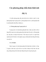
FIGURE 5.5 Example of the mass and its 3 × 3 neighborhood in a mammogram.

For simplicity, we take the square block with the length equal to the given radius
as the block of interest. We form a 3 × 3 neighborhood around the block of interest
and then estimate the AR model coefficients of each block, as shown in Figure 5.5.
The order of the AR model is assumed to be 1 × 1.
Copyright 2005 by Taylor & Francis Group, LLC