Finite element model for nonlinear analysis of steel–concrete composite beams using Timoshenkos beam theory
Bạn đang xem bản rút gọn của tài liệu. Xem và tải ngay bản đầy đủ của tài liệu tại đây (7.21 MB, 16 trang )
Finite element model for nonlinear analysis of steel–concrete composite
beams using Timoshenko's beam theory
Dinh Huynh Thai2) Bui Duc Vinh1) and Le Van Phuoc Nhan1)
1)
HCMUT, 268 Ly Thuong Kiet, Ho Chi Minh City, Viet Nam
Hoang Vinh TRCC, 270A Tay Thanh, Ho Chi Minh City, Viet Nam
1)
2)
ABSTRACT
This paper presents an analytical model for steel-concrete composite beams with partial shear
interaction and shear deformability of the two components. The model is obtained by coupling
the Timoshenko’s beam for the concrete slab and steel girder (T-T model). The nonlinear
material of concrete slab, steel girder and shear connectors are taken into account. The stiffness
matrix of the composite element with 16 DOFs is derived by the displacement based finite
element formulation. The numerical solutions are verified on simply supported and continuous
beams. The analytical results show good agreement with experimental data, they are also
compared with the difference models.
1. INTRODUCTION
Steel - concrete composite beams (CB) have been widely used in the construction industry
due to the advantages of combining the two materials. Modeling and analysis of steel–concrete
composite structures have been proposed in the literature (Spacone and El-Tawil 2004).
Newmark et al. (1951) analyzed CB with partial interaction. The Newmark model couples two
Euler–Bernoulli beams, i.e. one for the reinforced concrete (RC) slab and one for the steel
girder. Since then, many researchers have been extended the Newmark’s model (Gattesco 1999,
Dall’Asta and Zona 2002, Ranzi et al. 2004). Recently, Ranzi and Zona (2007) introduced a
beam model including the shear deformability of the steel component only. This model was
obtained by coupling an Euler–Bernoulli beam for the RC slab with a Timoshenko beam for the
steel girder. This parametric study was carried out using a locking-free finite element model
under the assumption of linear elastic materials and considering the time-dependent behaviour
of the concrete. Schnabl et al. (2007) presents an analytical solution and a FE formulation for
CB with coupled Timoshenko beams for both components, the material models are limited on
linear elastic behaviour. The results showed that shear deformations are more important for high
levels of shear connection degree, for short beams with small span-to-depth ratios, and for
beams with high elastic and shear modules ratios.
In this work,
w
the prroposed moddel is formuulated by couupling Timoshenko beam
ms for both the
RC slab annd steel girdder, it is refe
ferred as (T––T model). The
T governinng equations of CB moodel
with partiaal interactionn, based on kinematic assumptions
a
s substantiallly similar to
o the analytiical
solution was
w reportedd by Schnaabl et al. ((2007). Thee nonlinear behaviour of materiall is
consideredd for all com
mponents. Numerical
N
soolutions are obtained byy displacemeent-based finnite
element (F
FE). Four nu
umerical exaamples dealing with two simply suupported andd two two-sppan
continuouss CB are preesented.
2. ANALY
YTICAL MODEL
M
2.1 Moddel assumptiions
A typiccal steel–conncrete CB wiith prismaticc section is sh
hown in Figg. 1 (Ranzi annd Zona 20007).
An ortho normal
n
refereence system
m {O; X, Y, Z
Z} where i, j,
j k are the uunit vectors of
o axis X, Y,, Z.
The composite cross section
s
is foormed by thee concrete sllab, referredd to as Ac, and
a by the stteel
beam, refeerred to as As. The com
mposite actioon between the two com
mponents is provided byy a
continuouss deformablee shear conn
nection at thhe interface between
b
the two layers, whose dom
main
consists off the points in the YZ plane with y = ysc and z ∈ [0, L] . Thee main assum
mptions for the
T-T modell can be foun
nd in work of
o Schnabl ett al. (2007).
Fig.1 Typical compossite beam andd cross-sectiion
a strain fieelds
2.2 Dispplacement and
The dissplacement field
f
of a generic pointt P (x, y, z)) of the CB is defined by
b vector d as
shown in Eq.
E (1):
⎧dc ( y , z ) = v( z ) j + [ wc ( z ) + ( y − yc )ϕc ( z )]k
⎪
∀( x, y ) ∈ Ac , z ∈ [0, L]
⎪
(1)
d( y , z ) = ⎨
j
d
y
z
=
v
z
+
w
z
+
−
ϕ
(
z
)]
k
(
)
(
,
)
(
)
[
(
)
y
y
s
s
s
⎪ s
⎪⎩
∀( x, y ) ∈ As , z ∈ [0, L]
where v( z ) representts the defleection of booth componeents; wc ( z ) and ws ( z ) are the axxial
displacemeents of the reference
r
fibbers of the R
RC slab and the steel girrder, locatedd at yc and ys ,
respectivelly; ϕc ( z ) and ϕs ( z ) arre the rotattions of the top and boottom layerss, respectiveely.
Translation
ns and rotatiions are signned positive rrespectively
y as in Fig. 2 (Ranzi and Zona 2007).
The dissplacement field
f
can be grouped
g
in thhe vector:
uT ( z ) = [ wc ( z ) ws ( z ) v( z ) ϕc ( z ) ϕ s ( z ) ]
(2)
The slip betweenn the two componentss, which reepresents thhe discontinnuity of axxial
displacemeents at their interface, is given by veector s:
s( z ) = s ( z )k = ds ( ysc , z ) − dc ( ysc , z ) = [w s ( z ) − w c ( z ) − h s ϕ s ( z ) − h c ϕc ( z )]k
(3)
where hc = ysc − yc annd hs = ys − ysc
Fig..2 Displacem
ment field off the T–T com
mposite beam
m model
Based on
o the assum
med displacem
ment field, tthe non-zero componentss of the straiin field are:
⎧ε zzc ( y, z ) = w 'c + ( y − yc )ϕ 'c
⎪ ∀( x, y ) ∈ A , z ∈ [0, L]
∂d
⎪
c
ε z ( y, z ) = .k = ⎨
ε
y
z
=
w
(
,
)
'
∂z
s + ( y − ys )ϕ 's
⎪ zzs
⎪⎩ ∀( x, y ) ∈ As , z ∈ [0, L]
γ yzzc = v '+ ϕc
⎧
⎪∀( x, y ) ∈ A , z ∈ [0, L]
∂d
∂d
⎪
c
γ yz ( y, z ) = . j + .k = ⎨
γ
=
v
'+ ϕ s
∂z
∂y
yzzs
⎪
⎪⎩∀( x, y ) ∈ As , z ∈ [0, L]
(4)
(5)
where ε zc , ε zs and
γ yzc , γ yzs are the axial strains and the shear deformations of the two
components, respectively.
The strain field can be presented in the vector:
ε T ( z ) = ⎡⎣ε c ( z ) ε s ( z ) θ c ( z ) θ s ( z ) γ yzc ( z ) γ yzs ( z ) s ( z ) ⎤⎦
(6)
(6)
where ε c ( z ) = w 'c and ε s ( z ) = w 's are the axial strains at the levels of the reference fibres of the
two components respectively, θ c ( z ) = ϕ 'c and θ s ( z ) = ϕ 's is the curvature of the RC slab and the
steel girder.
The vector of strain functions can be obtained from the vector of displacement functions by
means of the relation:
(7)
ε = Du
where the matrix operator D is defined as:
⎡∂
⎢0
⎢
⎢0
⎢
D=⎢0
⎢0
⎢
⎢0
⎢ −1
⎣
0 0
0
∂ 0
0
0 0
0 0
∂
0
0 ∂
1
0 ∂
0
1 0 − hc
0 ⎤
0 ⎥⎥
0 ⎥
⎥
∂ ⎥
0 ⎥
⎥
1 ⎥
− hs ⎥⎦
(8)
being ∂ the derivative with respect to z .
2.3 Balance conditions
The principle of virtual work is utilized to obtain the weak form of the balance condition of
the problem:
^
∑
∫∫
α
L
Aα
= ∑∫
α
σ zα ε zα dAdz + ∑ ∫
L
L
α
∫
^
Aα
b. d dAdz + ∑ ∫
α
∂Aα
∫
^
Aα
^
τ yzα γ yzα dAdz + ∫ g sc s dz
L
(9)
^
t. d dsdz
where b and t are the body and surface force respectively; ( α = c, s ).
From Eq. (9) in weak form, the stress resultant entities, which are duals of the kinematic
entities derived from the assumed displacement field, can be identified and grouped in the vector
r:
rT = [ Nc
in which
Ns
Mc
M s Vc Vs
g sc ]
(10)
Nα = ∫ σ zα dAα
Aα
M α = ∫ σ zα ( y − yα )dAα
Aα
(11)
Vα = ∫ τ yzα dAα
Aα
Similarly, the external loads are written in the vector g:
gT = ⎡⎣ g zc
g zs
gy
mxs ⎤⎦
mxc
(12)
in which
g zα = ∫ b.kdAα + ∫
∂Aα
Aα
t.kds
g y = ∑ ∫ b.jdAα + ∑ ∫
∂Aα
Aα
t.jds
mxα = ∫ b.k ( yα − y )dAα + ∫
∂Aα
Aα
(13)
t.k ( yα − y ) s
Since Eq. (9) can be rewritten in compact form as:
∫
L
0
^
^
L
r.D udz = ∫ g.H udz
0
(14)
with the matrix operator H defined as:
⎡1
⎢0
⎢
H = ⎢0
⎢
⎢0
⎢⎣0
0
1
0
0
0
0
0
1
0
0
0
0
0
1
0
0⎤
0 ⎥⎥
0⎥
⎥
0⎥
1 ⎥⎦
(15)
3. MATERIAL MODELS
3.1 Concrete
The stress-strain relationship suggested by the CEB-FIB Model Code (2010) is adopted in
this paper for both compression and tension regions (Fig. 3). The σ c − ε c relationship is
approximated by the following functions:
• For ε c < ε c ,lim :
σc
f cm
⎛ k .η − η 2 ⎞
= − ⎜⎜
⎟⎟
⎝ 1 + ( k − 2 ) .η ⎠
(16)
where: η = ε c / ε c1 and k = Eci / Ec1
•
For σ ct ≤ 0.9 f ctm :
σ ct = Eci .ε ct
•
For 0.9 f ctm < σ ct ≤ f ctm :
(17)
⎛
σ ct = f cm . ⎜1 − 0.1
⎝
⎞
0.00015 − ε ct
⎟
00.00015 − 0.99 f ctm / Eci ⎠
(18)
(b)
(a))
Fig. 3 Sttress-strain diagram
d
for cconcrete: a) Compression, b) Tensio
on
(b)
(a)
m for steel, bb) Load-slip diagram forr stud shear connector
c
Fig. 4 a) Stress-strain diagram
3.2 Steeel
In the study,
s
the steel is modelled as an elaastic-perfecttly plastic material
m
incorrporating strrain
hardening.. Fig. 4 show
ws the stress--strain diagrram for steel in tension.
3.3 Sheear connectors
The connstitutive reelationship for
f the stud shear conneector was prroposed by Ollgaard et al.
(1971), is given by:
(
f scc = f max 1 − e
−β δ
)
α
with δ ≤ δ u
(19)
where fmaxx is the ultim
mate strengthh of the studd shear connnector; and α , β are coefficients to be
determinedd from test.
4. FINITE
E ELEMEN
NT FORMU
ULATION
unctions to approximate
a
e displacemeent are chooose. They arre must be the
The poolynomial fu
same ordeer in each displacement
d
t field, in faact that need
d to avoid the occurreence of lockking
problems:
f
(i) in axial strain (Eq. 4), the first derivvative of thee axial dispplacement w and the first
t rotationn ϕ must bbe polynom
mials of the same orderr to avoid the
derrivative of the
ecccentricity isssue (Gupta and
a Ma 19777, Erkmen annd Saleh 20112).
(ii) in the shear deeformation (Eq.
(
5), thee first derivaative of the ttransverse displacement
d
t v
n ϕ must bee polynomialls of the sam
me order in oorder to avoidd shear lockking
andd the rotation
(Yuunhua 1998,, Mukherjee and Prathapp 2001).
(iii) in the interfacce slip (Eq. 3), the axiaal displacem
ments w and the rotatioon ϕ must be
o
in ordder to avoid slip and cuurvature lockking (Dall’A
Asta
pollynomials off the same order
andd Zona 2004
4).
4.1 Thee displacemeent-based FE
E
The sim
mplest elemeent (Fig. 5a)) which can be derived for the T–T
T model has 10 degrees--offreedom (DOF).
(
Thaat is the at least requuired DOFss for descrribing the problem
p
unnder
considerattion. Its shappe functions are linear fuunctions for the axial dissplacements,, deflection and
a
rotations of
o componennts (Table 1).
Fig.5 Fiinite elementts for the T––T CB model
o the previo
ous considerrations, this ssimple 10 DOF FE does not satisfy the
t consistenncy
Based on
conditionss between th
he different displacemennt fields couupled in thee problem. The
T use of this
t
element caan lead to poor
p
and unnsatisfactory results. Th
hus, the use of the 10D
DOF T–T beeam
element is discouragedd.
Table 1: Degrees
D
of shhape functionns for the prroposed T–T
T finite elemeents
10D
DOF
16D
DOF
wc
ws
v
ϕc
ϕs
1
2
1
2
1
3
1
2
1
2
The FE
E fulfilling thhe consistenccy conditionns of the dispplacement fiield is the 166DOF depiccted
in Fig. 5b which enhannces the ordder of the approximated polynomialss to paraboliic functions for
the axial displacement
d
ts, rotations and
a to cubicc function forr transverse displacemennt (Table 1).
4.2 FE formulation
The displacement of the FE with a polynomial approximation of the displacement field is
written as:
(20)
u = Nd
and relation of displacement and strain as in Eq. (21):
ε = DNd = Bd
(21)
r = Dε = DBd
the Virtual Work Principle Eq. (9) becomes:
∫
L
0
^
L
^
DBd.Bd dz = ∫ g. H N d dz
(22)
0
Since, the following balance equation is obtained:
K e .d = fe
(23)
L
where K e = ∫ BT DBdz is stiffness matrix;
0
L
and fe = ∫ ( H N)T gdz is the vector of the internal nodal forces.
0
The calculation of load vector, internal nodal forces vector and stiffness matrix is performed
by means of numerical integration, using the trapezoidal rule through the thickness (the crosssection is subdivided into rectangular strips parallel to the x-axis) (Nguyen et al. 2009) and by
using the Gauss–Lobatto rule along the element length. In computer code, five Gauss points are
used in the 16DOF element. The non-linear balance equation can be written in iterative form
using the Newton–Raphson method.
5. NUMERICAL EXAMPLES
The numerical solutions of the proposed model are compared against experimental data
obtained by earlier experimental study. In the fact that, a group of two CB which material
limited in linear elastic range are investigated (Aribert et al. 1983 and Ansourian 1981). Other
group includes the simply-supported CB E1 tested by Chapman et al. (1964) and the two spans
CB CBI tested by Teraszkiewicz (1967) are considered for nonlinear analysis.
5.1 Simply supported steel–concrete CB (Aribert et al. 1983)
The proposed 16DOF beam element model is used to predict the elastic deflection of the
simply supported composite beam tested by Aribert et al.(1983). The geometric characteristics
and the material properties of the beam are shown in Fig. 6 and Table 2.
As shown in the figure a steel plate 120 × 8 mm is welded into bottom flange of the steel girder.
There are five rebars dia. of 14mm, placing in at the mid-depth of the RC slab.
Fig.6 Geometriccal characterristics of CB (Aribert et al. 1983)
The beeam is moddeled using six elemennts in order to comparee the performance of the
proposed model again
nst the exissting EB-EB
B 8DOF mo
odel (Dall’A
Asta and Zoona 2002) and
a
s
fouur elements are used, annd two morre elements are
experimenntal data. Beetween the supports,
placed at the
t beam endds.
Tablee 2: Mechaniical characteeristics of CB
B (Aribert ett al. 1983)
Param
meter
RC sllab
Steell girder
Distancee between thhe centroid of
o layer
and the layer interfaace
Area
hc = 50 mm
hs = 187 mm
m
mm2
Ac = 82310 m
As = 7220
0 mm2
Second moment of area
a
I c = 666.667 × 105 mm4
M
Ec = 20000 MPa
Pa
Gc = 8333 MP
I s = 1415 × 105 mm4
Es = 2000000 MPa
Gs = 8000
00 MPa
Elastic modulus
m
Shear modulus
m
Shear boond stiffnesss
k sc = 4500 MPa
s
the looad–deflectiion curve unnder the poiint load. It ccan be seen that numeriical
Fig. 7 shows
results of both modells are slighttly more flexxible than the
t test dataa. Howeverr, the proposed
model is closer to thhe experimeental data thhan the EB--EB 8DOF model, because the shhear
on of the cross-section
c
n is taken innto accountt for each llayer. Fig. 8 presents the
deformatio
comparisoon for the sliip distributio
on along thee beam leng
gth at load level
l
of 195 kN, the ressult
shows both
h models proovide almostt the identicaal slip distrib
bution.
Fiig.7 Load–deflection currves.
Fig.8 Slip distribbution alongg the beam.
m
deeflections obbtained withh the propossed model compared
c
w
with
Fig. 9 shows the mid-span
those obtained with EB
B-EB 8DOF
F model for ddifferent spaan-to-depth rratios (L/H) and shear boond
dicted by thee proposed model
m
is largger than the correspondding
stiffness (kksc). The defflection pred
one evaluaated accordiing to EB-E
EB 8DOF model,
m
for an
ny value of tthe ratio L/H
H. The curvves,
related to cases of low
wer shear stiiffness, monnotonically reeduce to thee case of abssent interacttion
Pa). It can bee seen that partial
p
interaaction resultss in a reducttion
(loose connnection withh ksc = 1 MP
of the effect of shear flexibility
f
off the connected memberss.
Fiig.9 Mid-spaan deflectionn versus the span-to-dept
s
th ratio
5.2 Twoo-span contiinuous compposite beam C
CTB6 (Ansourian 1981)
The prooposed modeel is now useed to simulatte a two-spaan continuouus steel–conccrete CB. Beeam
CTB6, whhich was a part of the experimenttal program carried outt by Ansourrian (1981),, is
consideredd. The geom
metric definition of thee beam is illlustrated in Fig. 10. The
T RC slabb is
longitudinnally reinforcced by rebarrs at the topp and bottom
m with differrent reinforccement ratioo in
the sagginng and hoggging region. The distancces from the interface to
t the bottoom and the top
rebars are 25 mm and 75 mm, respectively. T
The shear bonnd stiffness is assumed of 10,000 M
MPa
(Nguyen et
e al. 2011). The materiaal parameterrs used in thee computer analysis are Es = 210 GPa;
Gs = 80.76
6 GPa; Ec = 34
3 GPa; Gc = 14,167 GP
Pa.
Fig. 10 Geometrical
G
characteristtics of beam CTB6 (Anssourian 1981)
Fig.11 Load versu
us deflectionn curves.
Fig.12 Deflectionn curves alonng the beam
Two annalyses havee been carried out using the proposeed model. Thhe first one includes
i
an unu
cracked an
nalysis, in which
w
the cooncrete craccking in the slab is ignored. The second analyysis
comprises a ‘‘crackedd analysis’’, as suggested by Euro-ccode 4. The concrete craacking is takken
into accouunt by negleccting the con
ncrete contriibution along 15% of thhe span lengtth on each side
s
of the inteernal supporrt. The mid-span deflecttions obtaineed by the prroposed model, using four
fo
elements for
f the un-crracked analyysis and sixx elements for
fo the crackked analysis,, are compaared
against thhe experimenntal results in Fig. 11.. This figurre shows that the modeel predicts the
deflection curve with the ‘‘crackeed analysis’’ rather well. The resultss indicate thhat the concrrete
cracking effects
e
must be
b taken intoo account foor continuouss CB. Thesee effects can be seen cleaarly
in Fig. 12 with deflection curves along
a
the beaam.
5.3 Simp
mply supporteed steel–conncrete CB E11 (Chapman et al. 1964)
The nonlinear anallysis of simpply supporteed beam E1
1 was carried out, based
d on the tessted
beam of Chapman
C
et al.
a (1964). Shear
S
connecctors are heaaded studs (112.7 mm diaameter) in paairs
at 120 mm
m pitch. The geometric characteristi
c
cs, material properties and
a constituttive coefficiient
values of beam are shhown in Fig
g. 13, Tablee 3 and Tab
ble 4. The beam
b
is mod
deled using 22
elements: 20 elementss are used beetween the supports
s
and
d two elemeents are placed at the beeam
ends.
Fig.13 Geometrical characteristic
c
cs of beam E1
E
The nu
umerical sim
mulation is compared thee performan
nce of the prroposed model against the
data of Gaattesco (1999
9) and experrimental dataa. The load versus
v
mid-sspan deflectiion is plottedd in
Fig. 14 annd the valuess of slip at the
t steel–conncrete interfface along thhe beam axiss are plottedd in
Fig. 15 foor various lo
oading levelss. The plots show the good
g
agreem
ment between
n the analytiical
results andd the existinng data. The small differrences in thee slip curvess are likely due
d to the boond
relationshiip.
Table 3: Geometrical
G
characteristiics of beam E1
Span length (mm)
Concrete
C
slaab
Steel beam
Shear conneectors
Longitudina
L
al
reinforceme
r
nt
Thickness (m
T
mm)
W
Width
(mm)
S
Section
A (mm2)
Area
K
Kind
of studs
of studs
D
Distribution
N
Number
of sttuds
T (mm2)
Top
B
Bottom
(mm
m2)
5490
152.4
1220
12” x 6”” x 44lb/ft BSB
8400
12.7 x 50
Uniform
m in pairs
100
200
200
Tablee 4: Materiall properties aand constituttive coefficient values
Material
Concrete
Comprressive stren
ngth fc (MPa))
Tensilee strength fctt (MPa)
Peak sttrain in com
mpression ε c1
Peak sttrain in tensiion ε ct1
E1
32.7
7
3.07
7
0.0022
2
0.00015
5
CBI
466.7
3.89
0.0022
0.00015
Steel
Yield stress
s
(MPa))
Ultimaate tensile
stress (MPa)
(
Strain–
–harden
strain ε sh
Connectio
on
Elasticcity moduluss Es (MPa)
Strain–
–harden
moduluus Esh (MPa)
fmax (kN
N)
β (mm
m-1)
α
Fig.14 Loaad versus miid-span defleection curvees
Flang
ge
Web
Reinfforcement
Flang
ge
Web
Reinfforcement
Flang
ge
Web
Reinfforcement
250
0
297
7
320
0
465
5
460
0
320
0
0.00267
7
0.00144
4
206000
0
3500
0
301
301
321
470
470
485
0.012
0.012
0.010
206000
2500
66
6
0.8
8
0.45
5
322.4
4.72
1
1.0
Fig.15 Slip distribuution along sppan at variouus
loaad levels.
B CBI (Terasszkiewicz 19967)
5.4 Twoo-span contiinuous steel––concrete CB
In orderr to verify thhe numericall model in thhe presence of
o negative m
moments, coontinuous beeam
CBI, tested
d experimen
ntally by Terraszkiewicz (1967), werre simulated with the nuumerical moddel.
The geom
metric characcteristics, maaterial propeerties and coonstitutive coefficient
c
v
values
of beeam
CBI are sh
hown in Fig. 16, Table 4 and Table 55. In these siimulations bbonding was not considered
because th
he experimenntal beams were
w greasedd at the steel––concrete innterface to prrevent bondiing.
A total nuumber of 20 elements peer span weree used for beeam CBI. Ass the beam was
w symmetrric,
only one half
h of the beeam was mod
deled.
Fig.16 Geeometrical chharacteristics of beam CBI
metrical charracteristics of
o continuouss beam
Taable 5: Geom
Span length (mm)
Concrete
C
slaab
Steel beam
Shear conneectors
Longitudina
L
al
reinforceme
r
nt
Thickness (m
T
mm)
W
Width
(mm)
S
Section
A (mm2)
Area
K
Kind
of studs
P
Pitch
of studds (mm)
N
Number
of sttuds
H top (mm
Hog
m2)
H bottom (mm2)
Hog
S top (mm
Sag
m2)
S bottom ((mm2)
Sag
3354
60
610
6” x 3” x 12lb/ft BSB
8400
9.5 x 50
146
96
445
-
The com
mparison beetween somee results of tthe simulatio
on of beam C
CBI and thee correspondding
experimenntal results is
i shown in Fig.17, Figg.18 and Figg.19. In com
mpliance withh experimenntal
results theese quantities were plotted at P = 122 kN,, which corrresponds too 81% of the
experimenntal ultimate load at P = 150.5 kN. Inn those figurre, the experrimental resuults of the right
span are plotted
p
uponn the results of the left span to faccilitate compparison with
h the numeriical
results. Thhe plots show
w the good agreement
a
between the analytical
a
reesults and thee existing daata.
In Fig. 17, it can be noted
n
that thee curve of thhe analyticaal results liess almost alw
ways among the
experimenntal results of the two hallves of the bbeam.
Fig.17 Deflected shappe at load levvel of 122 kN
N
Fig.18
8 Slip distribbution along span at loadd
levell of 122 kN
Fiig.19 Strain profile alongg the span inn the bottom flange at load level of 122
1 kN
6. CONCLUSIONS
A numeerical modell for the lineear analysis and nonlineear analysis of steel–conncrete CB with
w
partial sheear interactio
on capable of
o accountinng for the shhear deformaability of booth componeents
has been presented.
p
T proposed
The
d model is fformulated by
b modelingg the RC slaab and the stteel
girder by means
m
of thee Timoshenkko beam moodels. The an
nalytical forrmulation haas been derivved
by means of
o the princiiple of virtuaal work. Thee numerical solution
s
has been obtained by meanss of
the displaccement-based FE methodd.
The nuumerical-expperimental co
omparisons validated thhe proposedd model reliability and the
capacity too determine the behavio
our of CB. The
T T-T mod
del gives a bbetter agreem
ment. Based on
these resuults, the effeects of shearr deformatioons need to be carefullyy evaluated for compossite
steel–conccrete system
ms, in particuular in the ccase the sm
mall length-too-depth ratio
o and large ksc
value. Furrthermore, th
he effect off concrete crracking in thhe hogging moment reggions has beeen
investigateed.
REFERENCES
Spacone, E. and El-Tawil, S. (2004), “Nonlinear analysis of steel–concrete composite structures: stateof-the-art”, J Struct Eng, 130 (2),159–168.
Newmark , N.M., Siess, C.P. and Viest , I.M. (1951), “Tests and analysis of composite beams with
incomplete interaction”, Proc Soc Exp Stress Anal, 9(1), 75–9.
Gattesco, N. (1999), “Analytical modeling of nonlinear behavior of composite beams with deformable
connection”, J Constr Steel Res, 52(2), 195-218.
Dall’Asta, A. and Zona, A. (2002), “Non-linear analysis of composite beams by a displacement
approach”, Comput Struct, 80(27–30), 2217–2228.
Ranzi, G., Bradford, M.A. and Uy, B. (2004), “A direct stiffness analysis of a composite beam with
partial interaction”, Int J Numer Methods Eng, 61(5), 657–672.
Ranzi , G. and Zona , A. (2007), “A steel–concrete composite beam model with partial interaction
including the shear deformability of the steel component, Eng Struct, 29(11), 3026–3041.
Schnabl , S., Saje , M., Turk, G. and Planinc, I. (2007), “Analytical solution of two-layer beam taking
into account interlayer slip and shear deformation”, J Struct Eng, 133(6), 886–894.
CEB-FIB Model code 2010, the International Federation for Structural Concrete.
Ollgaard, J.G., Slutter, R.G. and Fisher, J.W. (1971), “Shear strength of stud connectors in lightweight
and normal weight concrete”, AISC Eng J, 8(2), 55-64.
Gupta, A.K. and Ma, P.S. (1977), “Short communications. error in eccentric beam formulation”, Int J
Numer Methods Eng, 11, 1473-1483.
Erkmen, R.E. and Saleh, A. (2012), “Eccentricity effect in the finite element modeling of composite
beams”, Advances in Engineering Software, 52, 55-59.
Yunhua, L. (1998), “Explanation and elimination of shear locking and membrane locking with field
consistence approach”, Comput Methods Appl Mech Eng, 162 (1-4), 249-269.
Mukherjee, S. and Prathap ,G. (2001), “Analysis of shear locking in Timoshenko beam elements using
the function space approach”, Commun. Numer. Meth. Engng, 17 (6), 385-393.
Dall’Asta, A. and Zona, A. (2004), “Slip locking in finite elements for composite beams with deformable
shear connection”, Finite Elements in Analysis and Design, 40 (13-14), 1907-1930.
Nguyen, Q. H., Hjiaj, M., Uy, B. and Guezouli, S. (2009), “Analysis of composite beams in the hogging
moment regions using a mixed finite element formulation”, J Constr Steel Res, 65, 737-748.
Nguyen, Q.H., Martinelli, E. and Hjiaj, M. (2011), “Derivation of the exact stiffness matrix for a twolayer Timoshenko beam element with partial interaction”, Eng Struct, 33, 298-307.
Aribert, J.M., Labib, A.G. and Rival, J.C. (1983), “Etude numérique et expérimental de l’influence d’une
connexion partielle sur le comportement de poutres mixtes”. Communication présentée aux journées
AFPC. Mars. Thème 1, sous-thème.
Ansourian, P. (1981), “Experiments on continuous composite beams”, Proceedings of the Institution of
Civil Engineers, 71, 25-51.
Chapman, J.C. and Balakrishnan, S. (1964), “Experiments on composite beams”, Struct Eng, 42, 369–83.
Teraszkiewicz, J. (1967), “Static and fatigue behavior of simply supported and continuous composite
beams of steel and concrete”, PhD thesis: University of London.