Luyện thi GRE math review 4 data
Bạn đang xem bản rút gọn của tài liệu. Xem và tải ngay bản đầy đủ của tài liệu tại đây (4.27 MB, 109 trang )
GRADUATE RECORD EXAMINATIONS®
Math Review
Chapter 4: Data Analysis
Copyright © 2010 by Educational Testing Service. All rights
reserved. ETS, the ETS logo, GRADUATE RECORD
EXAMINATIONS, and GRE are registered trademarks of
Educational Testing Service (ETS) in the United States and other countries.
GRE Math Review 4 Data Analysis
1
®
The GRE Math Review consists of 4 chapters: Arithmetic, Algebra, Geometry, and
Data Analysis. This is the accessible electronic format (Word) edition of the Data
Analysis Chapter of the Math Review. Downloadable versions of large print (PDF) and
accessible electronic format (Word) of each of the 4 chapters of the Math Review, as well
as a Large Print Figure supplement for each chapter are available from the GRE
®
website. Other downloadable practice and test familiarization materials in large print and
accessible electronic formats are also available. Tactile figure supplements for the 4
chapters of the Math Review, along with additional accessible practice and test
familiarization materials in other formats, are available from E T S Disability Services
Monday to Friday 8:30 a m to 5 p m New York time, at 1-6 0 9-7 7 1-7 7 8 0, or
1-8 6 6-3 8 7-8 6 0 2 (toll free for test takers in the United States, U S Territories, and
Canada), or via email at
The mathematical content covered in this edition of the Math Review is the same as the
content covered in the standard edition of the Math Review. However, there are
differences in the presentation of some of the material. These differences are the result of
adaptations made for presentation of the material in accessible formats. There are also
slight differences between the various accessible formats, also as a result of specific
adaptations made for each format.
Information for screen reader users:
This document has been created to be accessible to individuals who use screen readers.
You may wish to consult the manual or help system for your screen reader to learn how
best to take advantage of the features implemented in this document. Please consult the
separate document, GRE Screen Reader Instructions.doc, for important details.
Figures
The Math Review includes figures. In accessible electronic format (Word) editions,
figures appear on screen. Following each figure on screen is text describing that figure.
Readers using visual presentations of the figures may choose to skip parts of the text
GRE Math Review 4 Data Analysis
2
describing the figure that begin with “Begin skippable part of description of …” and end
with “End skippable part of figure description.”
Mathematical Equations and Expressions
The Math Review includes mathematical equations and expressions. In electronic format
(Word) editions some of the mathematical equations and expressions are presented as
graphics. In cases where a mathematical equation or expression is presented as a graphic,
a verbal presentation is also given and the verbal presentation comes directly after the
graphic presentation. The verbal presentation is in green font to assist readers in telling
the two presentation modes apart. Readers using audio alone can safely ignore the
graphical presentations, and readers using visual presentations may ignore the verbal
presentations.
GRE Math Review 4 Data Analysis
3
Table of Contents
Table of Contents..............................................................................................................4
Overview of the Math Review............................................................................................5
Overview of this Chapter....................................................................................................5
4.1 Graphical Methods for Describing Data.......................................................................6
4.2 Numerical Methods for Describing Data...................................................................25
4.3 Counting Methods.......................................................................................................36
4.4 Probability...................................................................................................................49
4.5 Distributions of Data, Random Variables, and Probability Distributions.................58
4.6 Data Interpretation Examples.....................................................................................81
Data Analysis Exercises....................................................................................................91
Answers to Data Analysis Exercises .............................................................................105
GRE Math Review 4 Data Analysis
4
Overview of the Math Review
The Math Review consists of 4 chapters: Arithmetic, Algebra, Geometry, and Data
Analysis.
Each of the 4 chapters in the Math Review will familiarize you with the mathematical
skills and concepts that are important to understand in order to solve problems and reason
®
quantitatively on the Quantitative Reasoning measure of the GRE revised General Test.
The material in the Math Review includes many definitions, properties, and examples, as
well as a set of exercises with answers at the end of each chapter. Note, however that this
review is not intended to be all inclusive. There may be some concepts on the test that are
not explicitly presented in this review. If any topics in this review seem especially
unfamiliar or are covered too briefly, we encourage you to consult appropriate
mathematics texts for a more detailed treatment.
Overview of this Chapter
This is the Data Analysis Chapter of the Math Review.
The goal of data analysis is to understand data well enough to describe past and present
trends, predict future events, and make good decisions. In this limited review of data
analysis, we begin with tools for describing data; follow with tools for understanding
counting and probability; review the concepts of distributions of data, random variables,
and probability distributions; and end with examples of interpreting data.
GRE Math Review 4 Data Analysis
5
4.1 Graphical Methods for Describing Data
Data can be organized and summarized using a variety of methods. Tables are commonly
used, and there are many graphical and numerical methods as well. The appropriate type
of representation for a collection of data depends in part on the nature of the data, such as
whether the data are numerical or nonnumerical. In this section, we review some
common graphical methods for describing and summarizing data.
Variables play a major role in algebra because a variable serves as a convenient name for
many values at once, and it also can represent a particular value in a given problem to
solve. In data analysis, variables also play an important role but with a somewhat
different meaning. In data analysis, a variable is any characteristic that can vary for the
population of individuals or objects being analyzed. For example, both gender and age
represent variables among people.
Data are collected from a population after observing either a single variable or observing
more than one variable simultaneously. The distribution of a variable, or distribution of
data, indicates the values of the variable and how frequently the values are observed in
the data.
Frequency Distributions
The frequency, or count, of a particular category or numerical value is the number of
times that the category or value appears in the data. A frequency distribution is a table
or graph that presents the categories or numerical values along with their associated
frequencies. The relative frequency of a category or a numerical value is the associated
frequency divided by the total number of data. Relative frequencies may be expressed in
terms of percents, fractions, or decimals. A relative frequency distribution is a table or
graph that presents the relative frequencies of the categories or numerical values.
GRE Math Review 4 Data Analysis
6
Example 4.1.1: A survey was taken to find the number of children in each of 25
families. A list of the 25 values collected in the survey follows.
1
3
4
3
3
2
3
5
2
0
0
1
2
4
2
4
2
3
1
3
1
0
2
2
1
The resulting frequency distribution of the number of children is presented in a 2
column table in Data Analysis Figure 1 below. The title of the table is “Frequency
Distribution”. The heading of the first column is “Number of Children” and the
heading of the second column is “Frequency”.
Frequency Distribution
Number of Children
Frequency
0
3
1
5
2
7
3
6
4
3
5
1
Total
25
Data Analysis Figure 1
The resulting relative frequency distribution of the number of children is presented in
a 2 column table in Data Analysis Figure 2 below. The title of the table is “Relative
GRE Math Review 4 Data Analysis
7
Frequency Distribution”. The heading of the first column is “Number of Children”
and the heading of the second column is “Relative Frequency”.
Relative Frequency Distribution
Number of Children
Relative Frequency
0
12%
1
20%
2
28%
3
24%
4
12%
5
4%
Total
100%
Data Analysis Figure 2
Note that the total for the relative frequencies is 100%. If decimals were used instead
of percents, the total would be 1. The sum of the relative frequencies in a relative
frequency distribution is always 1.
Bar Graphs
A commonly used graphical display for representing frequencies, or counts, is a bar
graph, or bar chart. In a bar graph, rectangular bars are used to represent the categories
of the data, and the height of each bar is proportional to the corresponding frequency or
relative frequency. All of the bars are drawn with the same width, and the bars can be
presented either vertically or horizontally. Bar graphs enable comparisons across several
categories, making it easy to identify frequently and infrequently occurring categories.
GRE Math Review 4 Data Analysis
8
Example 4.1.2: A bar graph entitled “Fall 2009 Enrollment at Five Colleges” is
shown in Data Analysis Figure 3 below. The bar graph has 5 vertical bars, one for
each of 5 colleges.
Data Analysis Figure 3
Begin skippable part of description of Data Analysis Figure 3.
The vertical axis of the bar graph is labeled “Enrollment”. There are horizontal
gridlines at multiples of 1,000, from 0 to 8,000, and tick marks halfway between each
of the horizontal gridlines. Along the horizontal axis are the 5 colleges: College A,
GRE Math Review 4 Data Analysis
9
College B, College C, College D, and College E. The graph contains a vertical bar for
each of the five colleges. The bars are as follows.
College A: The top of the bar is at 4,000.
College B: The top of the bar is halfway between 4,000 and 5,000, which is about
4,500.
College C: The top of the bar is a little below 5,000.
College D: The top of the bar is a little below the tick mark halfway between 6,000
and 7,000; that is to say, the top of the bar is a little below 6,500.
College E: The top of the bar is halfway between 7,000 and 8,000, which is about
7,500.
End skippable part of figure description.
From the graph, we can conclude that the college with the greatest fall 2009
enrollment was College E, and the college with the least enrollment was College A.
Also, we can estimate that the enrollment for College D was about 6,400.
A segmented bar graph is used to show how different subgroups or subcategories
contribute to an entire group or category. In a segmented bar graph, each bar represents a
category that consists of more than one subcategory. Each bar is divided into segments
that represent the different subcategories. The height of each segment is proportional to
the frequency or relative frequency of the subcategory that the segment represents.
Example 4.1.3: Data Analysis Figure 4 below is a modified version of Data Analysis
Figure 3. All features of Data Analysis Figure 3 are in Data Analysis Figure 4, except
that each of the bars in Data Analysis Figure 4 is divided into two segments. The two
segments represent full time students and part time students.
GRE Math Review 4 Data Analysis
10
Data Analysis Figure 4
Begin skippable part of description of Data Analysis Figure 4.
The lower segment of each bar represents part time students, and the upper segment
of each bar represents full time students. The segmented bars for each college are as
follows.
College A: The part time student segment of the bar goes from 0 to 1,000; and the full
time student segment goes from 1,000 to 4,000.
College B: The part time student segment of the bar goes from 0 to about 1,500; and
the full time student segment goes from about 1,500 to about 4,500.
GRE Math Review 4 Data Analysis
11
College C: The part time student segment of the bar goes from 0 to about 2,500; and
the full time student segment goes from about 2,500 to a little below 5,000.
College D: The part time student segment of the bar goes from 0 to a number
between 2,000 and 2,500 (a little closer to 2,000 than to 2,500); and the full time
student segment goes from a number between 2,000 and 2,500 (a little closer to 2,000
than to 2,500) to a little below 6,500.
College E: The part time student segment of the bar goes from 0 to about 3,500; and
the full time student segment goes from about 3,500 to about 7,500.
End skippable part of figure description.
The total enrollment, the full time enrollment, and the part time enrollment at the 5
colleges can be estimated from the segmented bar graph in Data Analysis Figure 4.
For example, for College D, the total enrollment was a little below 6,500 or
approximately 6,400 students, the part time enrollment was approximately 2,200, and
the full time enrollment was approximately
4,200 students.
6,400 minus 2,200, or
Bar graphs can also be used to compare different groups using the same categories.
Example 4.1.4: A bar graph entitled “Fall 2009 and Spring 2010 Enrollment at Three
Colleges” is shown in Data Analysis Figure 5 below. The bar graph has 3 pairs of
vertical bars, one pair for each of three colleges. The left bar of each pair corresponds
to the number of students enrolled in Fall 2009, and the right bar corresponds to the
number of students enrolled in Spring 2010.
GRE Math Review 4 Data Analysis
12
Data Analysis Figure 5
Begin skippable part of description of Data Analysis Figure 5.
The vertical axis of the bar graph is labeled “Enrollment”. There are horizontal
gridlines at multiples of 1,000, from 0 to 6,000. Along the horizontal axis are the 3
colleges: College A, College B, and College C.
The pairs of bars for each college are as follows.
College A: The top of the Fall 2009 bar is at 4,000. The top of the Spring 2010 bar is a
little below 4,000. The difference between the top of the Fall 2009 bar and the Spring
2010 bar is roughly 250.
College B: The top of the Fall 2009 bar is halfway between 4,000 and 5,000, which is
about 4,500. The top of the Spring 2010 bar is a little below 4,000, at the same height
GRE Math Review 4 Data Analysis
13
as the top of the Spring 2010 bar for College A. The difference between the top of the
Fall 2009 bar and the Spring 2010 bar is a little more than 500.
College C: The top of the Fall 2009 bar is a little below 5,000. The top of the Spring
2010 bar is a little below 5,000, slightly below the top of the Fall 2009 bar. The
difference between the top of the Fall 2009 bar and the Spring 2010 bar is less than
100.
End skippable part of figure description.
Observe that for all three colleges, the Fall 2009 enrollment was greater than the
Spring 2010 enrollment. Also, the greatest decrease in the enrollment from Fall 2009
to Spring 2010 occurred at College B.
Although bar graphs are commonly used to compare frequencies, as in the examples
above, they are sometimes used to compare numerical data that could be displayed in a
table, such as temperatures, dollar amounts, percents, heights, and weights. Also, the
categories sometimes are numerical in nature, such as years or other time intervals.
Circle Graphs
Circle graphs, often called pie charts, are used to represent data with a relatively small
number of categories. They illustrate how a whole is separated into parts. The data is
presented in a circle such that the area of the circle representing each category is
proportional to the part of the whole that the category represents.
Example 4.1.5: A circle graph is shown in Data Analysis Figure 6 below. The title of
the graph is “United States Production of Photographic Equipment and Supplies in
1971”. There are 6 categories of photographic equipment and supplies represented in
the graph.
GRE Math Review 4 Data Analysis
14
Data Analysis Figure 6
Begin skippable part of description of Data Analysis Figure 6.
In the figure it is given that the total United States Production of Photographic
Equipment and Supplies was $3,980 million. By category, the percents given in the
graph are as follows.
Sensitized Goods:
Office Copiers:
47%
25%
Microfilm Equipment: 4%
GRE Math Review 4 Data Analysis
15
Prepared Photochemicals: 7%
Still Picture Equipment: 12%
Motion Picture Equipment: 5%
End skippable part of figure description.
From the graph you can see that Sensitized Goods was the category with the greatest
dollar value.
Each part of a circle graph is called a sector. Because the area of each sector is
proportional to the percent of the whole that the sector represents, the measure of the
central angle of a sector is proportional to the percent of 360 degrees that the sector
represents. For example, the measure of the central angle of the sector representing the
category Prepared Photochemicals is 7 percent of 360 degrees, or 25.2 degrees.
Histograms
When a list of data is large and contains many different values of a numerical variable, it
is useful to organize it by grouping the values into intervals, often called classes. To do
this, divide the entire interval of values into smaller intervals of equal length and then
count the values that fall into each interval. In this way, each interval has a frequency and
a relative frequency. The intervals and their frequencies (or relative frequencies) are often
displayed in a histogram. Histograms are graphs of frequency distributions that are
similar to bar graphs, but they have a number line for the horizontal axis. Also, in a
histogram, there are no regular spaces between the bars. Any spaces between bars in a
histogram indicate that there are no data in the intervals represented by the spaces.
An example of a histogram for data grouped into a large number of classes is given later
in this chapter (Example 4.5.1 in Section 4.5).
GRE Math Review 4 Data Analysis
16
Numerical variables with just a few values can also be displayed using histograms, where
the frequency or relative frequency of each value is represented by a bar centered over
the value.
Example 4.1.6: In Data Analysis Figure 2, the relative frequency distribution of the
number of children of each of 25 families was displayed as a 2 column table. For your
convenience, Data Analysis Figure 2 is repeated below.
Relative Frequency Distribution
Number of Children
Relative Frequency
0
12%
1
20%
2
28%
3
24%
4
12%
5
4%
Total
100%
Data Analysis Figure 2 (repeated)
This relative frequency distribution can also be displayed as a histogram as shown in
Data Analysis Figure 7 below.
GRE Math Review 4 Data Analysis
17
Data Analysis Figure 7
Begin skippable part of description of Data Analysis Figure 7.
The title of the histogram is “Relative Frequency Distribution”. The vertical axis of
the histogram is labeled “Relative Frequency”. There are 6 equally spaced horizontal
gridlines representing relative frequencies from 5% to 30%, in increments of 5%. The
horizontal axis of the histogram is labeled “Number of Children” and the numbers 0,
1, 2, 3, 4, and 5 are equally spaced along the horizontal axis. Centered above each of
these 6 numbers of children is a vertical bar representing the relative frequency of that
number of children. All of the bars have the same width. The bars are as follows:
For 0 children: The top of the bar is between 10% and 15% (a little closer to 10% than
to 15%).
For 1 child: The top of the bar is at 20%.
For 2 children: The top of the bar is between 25% and 30% (a little closer to 30% than
to 25%).
For 3 children: The top of the bar is a little below 25%.
GRE Math Review 4 Data Analysis
18
For 4 children: The top of the bar for 4 children and the top of the bar for 0 children
are the same height; that is, the top of these bars is between 10% and 15%, a little
closer to 10% than to 15%.
For 5 children: The top of the bar is a little below 5%.
End skippable part of figure description.
Histograms are useful for identifying the general shape of a distribution of data. Also
evident are the “center” and degree of “spread” of the distribution, as well as high
frequency and low frequency intervals. From the histogram in Data Analysis Figure 7
above, you can see that the distribution is shaped like a mound with one peak; that is, the
data are frequent in the middle and sparse at both ends. The central values are 2 and 3,
and the distribution is close to being symmetric about those values. Because the bars all
have the same width, the area of each bar is proportional to the amount of data that the
bar represents. Thus, the areas of the bars indicate where the data are concentrated and
where they are not.
Finally, note that because each bar has a width of 1, the sum of the areas of the bars
equals the sum of the relative frequencies, which is 100% or 1, depending on whether
percents or decimals are used. This fact is central to the discussion of probability
distributions later in this chapter.
Scatterplots
All examples used thus far have involved data resulting from a single characteristic or
variable. These types of data are referred to as univariate; that is, data observed for one
variable. Sometimes data are collected to study two different variables in the same
population of individuals or objects. Such data are called bivariate data. We might want
to study the variables separately or investigate a relationship between the two variables. If
the variables were to be analyzed separately, each of the graphical methods for univariate
data presented above could be applied.
GRE Math Review 4 Data Analysis
19
To show the relationship between two numerical variables, the most useful type of graph
is a scatterplot. In a scatterplot, the values of one variable appear on the horizontal axis
of a rectangular coordinate system and the values of the other variable appear on the
vertical axis. For each individual or object in the data, an ordered pair of numbers is
collected, one number for each variable, and the pair is represented by a point in the
coordinate system.
A scatterplot makes it possible to observe an overall pattern, or trend, in the relationship
between the two variables. Also, the strength of the trend as well as striking deviations
from the trend are evident. In many cases, a line or a curve that best represents the trend
is also displayed in the graph and is used to make predictions about the population.
Example 4.1.7: A bicycle trainer studied 50 bicyclists to examine how the finishing
time for a certain bicycle race was related to the amount of physical training in the
three months before the race. To measure the amount of training, the trainer
developed a training index, measured in “units” and based on the intensity of each
bicyclist’s training. The data and the trend of the data, represented by a line, are
displayed in the scatterplot in Data Analysis Figure 8 below.
GRE Math Review 4 Data Analysis
20
Data Analysis Figure 8
Begin skippable part of description of Data Analysis Figure 8.
The horizontal axis of the scatterplot is labeled “Training Index (units)” and includes
units from 0 to 100, in increments of 10. The vertical axis is labeled “Finishing Time
(hours)” and includes the time 0.0 and the times from 3.0 to 6.0, in increments of 0.5.
The scatterplot contains 50 data points and a trend line. From the figure it can be
GRE Math Review 4 Data Analysis
21
estimated that the trend line passes through the points
0 comma 5.8, 30 comma
5.0, 50 comma 4.5, 70 comma 4.0, and 100 comma 3.2.
End skippable part of figure description.
When a trend line is included in the presentation of a scatterplot, it shows how
scattered or close the data are to the trend line, or to put it another way, how well the
trend line fits the data. In the scatterplot in Data Analysis Figure 8 above, almost all of
the data points are close to the trend line. The scatterplot also shows that the finishing
times generally decrease as the training indices increase.
Several types of predictions can be based on the trend line. For example, it can be
predicted, based on the trend line, that a bicyclist with a training index of 70 units
would finish the race in approximately 4 hours. This value is obtained by noting that
the vertical line at the training index of 70 units intersects the trend line very close to
4 hours.
Another prediction based on the trend line is the number of minutes that a bicyclist
can expect to lower his or her finishing time for each increase of 10 training index
units. This prediction is basically the ratio of the change in finishing time to the
change in training index, or the slope of the trend line. Note that the slope is negative.
To estimate the slope, estimate the coordinates of any two points on the line. For
instance, the points at the extreme left and right ends of the line:
0 comma 5.8 and 100 comma 3.2. The slope can be computed
as follows:
the fraction with numerator 3.2 minus 5.8, and
denominator 100 minus 0 = negative 2.6 over 100, which is equal to negative 0.026,
GRE Math Review 4 Data Analysis
22
which is measured in hours per unit. The slope can be interpreted as follows: the
finishing time is predicted to decrease 0.026 hours for every unit by which the
training index increases. Since we want to know how much the finishing time
decreases for an increase of 10 units, we multiply the rate by 10 to get 0.26 hour per
10 units. To compute the decrease in minutes per 10 units, we multiply 0.26 by 60 to
get approximately 16 minutes. Based on the trend line, the bicyclist can expect to
decrease the finishing time by 16 minutes for every increase of 10 training index
units.
Time Plots
Sometimes data are collected in order to observe changes in a variable over time. For
example, sales for a department store may be collected monthly or yearly. A time plot
(sometimes called a time series) is a graphical display useful for showing changes in data
collected at regular intervals of time. A time plot of a variable plots each observation
corresponding to the time at which it was measured. A time plot uses a coordinate plane
similar to a scatterplot, but the time is always on the horizontal axis, and the variable
measured is always on the vertical axis. Additionally, consecutive observations are
connected by a line segment to emphasize increases and decreases over time.
Example 4.1.8: This example is based on the time plot entitled “Fall Enrollment for
College A, 2001 to 2009”, which is shown in Data Analysis Figure 9 below.
GRE Math Review 4 Data Analysis
23
Data Analysis Figure 9
Begin skippable part of description of Data Analysis Figure 9.
The horizontal axis of the time plot is labeled “Year” and contains the years from
2001 to 2009. The vertical axis is labeled “Enrollment” and contains the numbers
from 0 to 5,000, in increments of 1,000. In fall 2001 the enrollment was
approximately 1,200 and in fall 2009 the enrollment was approximately 4,000. The
change in fall enrollment between consecutive years was less than 1,000, except for
the change in enrollment between fall 2008 to fall 2009, which was a little over 1,000.
End skippable part of figure description.
The time plot shows that the greatest increase in fall enrollment between consecutive
years was the change between 2008 to 2009. The slope of the line segment joining the
values for 2008 and 2009 is greater than the slopes of the line segments joining all
other consecutive years, because the time intervals are regular.
Although time plots are commonly used to compare frequencies, as in Example 4.1.8
above, they can be used to compare any numerical data as the data change over time,
such as temperatures, dollar amounts, percents, heights, and weights.
GRE Math Review 4 Data Analysis
24
4.2 Numerical Methods for Describing Data
Data can be described numerically by various statistics, or statistical measures. These
statistical measures are often grouped in three categories: measures of central tendency,
measures of position, and measures of dispersion.
Measures of Central Tendency
Measures of central tendency indicate the “center” of the data along the number line and
are usually reported as values that represent the data. There are three common measures
of central tendency:
1. the arithmetic mean—usually called the average or simply the mean,
2. the median, and
3. the mode.
To calculate the mean of n numbers, take the sum of the n numbers and divide it by n.
Example 4.2.1: For the five numbers 6, 4, 7, 10, and 4, the mean is
the fraction with numerator 6 + 4 + 7 + 10 + 4, and
denominator 5 = 31 over 5, which is equal to 6.2.
When several values are repeated in a list, it is helpful to think of the mean of the
numbers as a weighted mean of only those values in the list that are different.
GRE Math Review 4 Data Analysis
25