AAE556 Lecture_3435_pk_flutter
Bạn đang xem bản rút gọn của tài liệu. Xem và tải ngay bản đầy đủ của tài liệu tại đây (276.12 KB, 41 trang )
AAE 556
Aeroelasticity
The P-k flutter solution method
(also known as the “British” method)
Purdue Aeroelasticity
1
The eigenvalue problem from the Lecture 33
ωh2
ω
2 ÷ 0 h b 1
−
+
÷( 1 + ig ) ωθ
ω
θ xθ
2
0
rθ
2
θ
2
1 Lh
+
µ
M θ h
ωθ2
0
h ω 2 ÷
1
Ω 2 b = h
x
1
θ 0
θ
rθ 2
xθ h
b
2
rθ θ
1
h
L
−
+
a
÷Lh b = 0
α 2
0
θ
M θθ
xθ 1 Lh
+
rθ 2 µ
M θ h
1
h
Lα − 2 + a ÷Lh b
θ
M θθ
2
Purdue Aeroelasticity
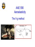
Genealogy of the V-g or “k” method
i
Equations of motion for harmonic response (next slide)
–
–
–
i
Forcing frequency and airspeeds are is known parameters
Reduced frequency k is determined from ω and V
Equations are correct at all values of ω and V.
Take away the harmonic applied forcing function
–
–
–
Equations are only true at the flutter point
We have an eigenvalue problem
Frequency and airspeed are unknowns, but we still need k to define the numbers to compute the
elements of the eigenvalue problem
–
We invent ed Theodorsen’s method or V-g artificial damping to create an iterative approach to finding
the flutter point
Purdue Aeroelasticity
3
Go back to the original typical section equations of motion, restricted to steady-state
harmonic response
2 AEOM
+ω
DEOM
h
BEOM F
b =
EEOM M SC
θ
4
Purdue Aeroelasticity
The coefficients for the EOM’s
AEOM
ω 2 ω 2 L
= − 1 − h ÷ θ2 ÷− h
ωθ ω ÷ µ
BEOM
DEOM
1
1
= − xθ − Lα − Lh + a ÷÷
µ
2
1
1
= − xθ − M h − Lh + a ÷÷
µ
2
(
EEOM = − rθ2 1 − ωθ2
)
Mh
+
µ
2
1
M α Lα 1
Lh 1
+
a
−
+
+
a
−
+
a
÷
÷
÷
2
µ
µ
2
µ
2
5
Purdue Aeroelasticity
The eigenvalue problem
2 AEOM
ω
DEOM
h
BEOM 0
b =
EEOM 0
θ
AEOM
DEOM
h
BEOM 0
b =
EEOM 0
θ
AEOM
( −µ )
DEOM
h
BEOM 0
b =
EEOM 0
θ
ω
ω2
2
6
Purdue Aeroelasticity
Another version of the eigenvalue problem with different
coefficents
AEOM
( −µ )
DEOM
h
h
BEOM
A B 0
b =
b =
EEOM D E 0
θ
θ
ω 2 ω 2 ω 2
A = µ 1 − h ÷ θ ÷ h ÷ ( 1 + ig ) ÷+ Lh
ωθ ω ωθ
÷
1
B = µ xθ + Lα − Lh + a ÷
2
7
Purdue Aeroelasticity
Definitions of terms for alternative set-up of eigenvalue equations for
“k-method”
h
A B 0
b =
D E θ 0
1
D = µ xθ + M h − Lh + a ÷
2
2
ω
θ
1
2
E = µ rθ 1 −
1
+
ig
÷−
M
+
a
+ Mα
(
)
h
÷
ω ÷
÷
2
2
1
1
− Lα + a ÷+ Lh + a ÷
2
2
8
Purdue Aeroelasticity
Return to the EOM’s before we assumed harmonic motion
Here is what we would like to have
&j } + K ij { η j } + Aij( 1) { η j } + Aij( 2) { η&j } + Aij( 3) { η&
&
M ij { η&
j } = { 0}
{η } = {η } e
j
j
Here is the first step in solving the stability problem
pt
p = σ + jω
p 2 M ij { η j } + Kij { η j } + Aij( 1) { η j }
2
3
+ p Aij( ) { η j } + p 2 Aij( ) { η j } = { 0}
9
Purdue Aeroelasticity
The p-k method will use the harmonic aero results to cast the stability
problem in the following form
1
p M ij { η } − p Bij { η } + K ij − ρV 2 Qij ,real { η } = { 0}
2
2
{η ( t )} = {η} e
…but first, some preliminaries
Purdue Aeroelasticity
10
pt
Revisit the original, harmonic EOM’s where the aero forces were still on the right hand side
of the EOM’s and we hadn’t yet nondimensionalized
h
1
iωt
P = − L = πρ b ω Lh ÷+ Lα − + a ÷Lh θ e
2
b
3
2
1
h b iωt
Lα − 2 + a ÷Lh ÷ e
θ
P = πρ b ω ( Lh )
3
2
h
V
airfoil chordline
b
ba
shear center
b
P
P = A11
h
A12 b
θ
11
Purdue Aeroelasticity
This lift expression looks strange; where is the dynamic
pressure?
h
1
iωt
P = πρ b ω Lh ÷+ Lα − + a ÷Lh θ e
2
b
3
2
V 2
h
i ωt
1
3 2
P = 2 πρb ω Lh + Lα − + a Lh θ e
2
V
b
ρV 2
b 2ω 2
P=
b( 2π ) 2
2
V
ωb
k=
V
Purdue Aeroelasticity
12
h
1
i ωt
Lh + Lα − + a Lh θ e
2
b
Writing aero force in different notation
- more term definitions
P = A11
h 1
h
2
A12 b = ρV Q11 Q12 b
θ 2
θ
Q11
Q11
2
A
Q12 =
2 11
ρV
2πρ b3ω 2
Q12 =
( Lh )
2
ρV
A12
1
Lα − + a ÷Lh ÷
2
The Qij’s are complex numbers
13
Purdue Aeroelasticity
Aero force
in terms of the Qij’s
Q11
Q12 = 2bπ k ( Lh )
1
Lα − Lh + a ÷÷
2
2
(
Q11 = 2π bk 2 Lh = 2π b k 2 − i 2kC ( k )
)
1
Q12 = 2π bk Lα − Lh + a ÷÷
2
2
k2
1
2
Q12 = 2π b − ik ( 1 + 2C ( k ) ) − 2C ( k ) ÷− k − i 2kC ( k ) + a ÷÷
2
2
÷
(
)
14
Purdue Aeroelasticity
Q11
Focus first on the term
(
Q11 = 2π b k − i 2kC ( k )
2
(
Q11 = 2π b k 2 − i 2k ( F + iG )
(
)
Q11 = 2π b k 2 + 2kG − i [ 2kF ]
)
Q11 = Q11,real + iQ11,imaginary
15
Purdue Aeroelasticity
)
The second term
k2
1
2
Q12 = 2π b − ik ( 1 + 2C ( k ) ) − 2C ( k ) ÷− k − i 2kC ( k ) + a ÷÷
2
2
÷
(
)
k2
1
2
Q12 = 2π b − ik ( 1 + 2 ( F + iG ) ) − 2 ( F + iG ) ÷− k − i 2k ( F + iG ) + a ÷÷
2
2
÷
(
)
3
1
2
Q12 = 2π b −2 F − k a + 2kG + a ÷+ i −k − 2G + 2kF − + a ÷÷÷÷
2
2
÷
16
Purdue Aeroelasticity
Let’s adopt notation from the controls community to help with our
conversion
(
Q11 = 2π b k 2 + 2kG − j [ 2kF ]
)
Q11 = Q11,real + jQ11,imaginary
If we were to assume motion e pt and p ≅ jω
p
then
≅1
jω
Q11 = Q11,real
p
+
÷ jQ11,imaginary
jω
17
Purdue Aeroelasticity
Continue working on the first term in the aero force expression
p
Q11 = Q11,real + ÷Q11,imaginary
ω
Q11,imaginary
Q11 = Q11,real + p
ω
P = A11
h
A12 b
θ
The expression for A11 reads
2
1
1
ρ
V
A11 = ρV 2Q11,real + p
Q11,imaginary
2
2 ω
18
Purdue Aeroelasticity
The term with the p in it looks like a damping term so let’s work on it
2
1
1
ρ
V
A11 = ρV 2Q11,real + p
Q11,imaginary
2
2 ω
1
ρVb V
2
A11 = ρV Q11, real + p
Q11,imaginary
2
2 bω
1
ρVb Q11,imaginary
2
A11 = ρV Q11,real + p
2
2
k
19
Purdue Aeroelasticity
Finally, the exact expressions for each term are as follows
1
ρVb Q11,imaginary
2
A11 = ρV Q11,real + p
2
2
k
(
Q11 = 2π b k 2 + 2kG − j [ 2kF ]
)
1
ρVb
2
2
A11 = ρV 2π b k + 2kG − p
[ 2F ]
2
2
Both terms are real numbers, there is no j here.
20
Purdue Aeroelasticity
Aerodynamic moment expression
M aero
Mα =
1 1
h
− + a ÷Lh ÷
b
2 2
4 2
= πρ b ω
2
+ M α − Lα + 1 ÷ 1 + a ÷+ Lh 1 + a ÷ ÷θ
÷
2
2
2
3 1
−i
8 k
M aero = A21
h
A22 b
θ
1 1
A21 = πρ b 4ω 2 − + a ÷Lh ÷
2 2
2
1
1
1
4 2
A22 = πρ b ω M α − Lα + ÷ + a ÷+ Lh + a ÷ ÷
2 2
2
÷
21
Purdue Aeroelasticity
÷
÷
÷
÷
÷
The Qij’s
2
Q21 Q22 =
A
2 21
ρV
Q21,real
2
= Real
A
2 21 ÷
ρV
Q22,real
2
= Real
A
2 22 ÷
ρV
A22
Q21,imaginary
2
= Imag
A
2 21 ÷
ρV
Q22,imaginary
2
= Imag
A
2 22 ÷
ρV
22
Purdue Aeroelasticity
The p-k process
i
Step 1
i
Choose a value of k and compute all four complex aerodynamic
coefficients
– These are the complex Aij’s with the Theodorsen Circulation function in
them
– These will be a set of complex numbers, not algebraic expressions
i
Choose an air density (altitude) and airspeed (V)
Purdue Aeroelasticity
23
Perform this computation
2
Qij =
A
2 ij
ρV
24
Purdue Aeroelasticity
Compute the aerodynamic damping matrix, defined as
1 Vb
Bij = ρ
Qij ,imaginary
2 k
Qij ,imaginary
1
Bij = ρVb
2
k
25
Purdue Aeroelasticity