Introduction – Equations of motion G. Dimitriadis 03

Aeroelasticity
Lecture 3:
Unsteady Aerodynamics –
Theodorsen
G. Dimitriadis
Introduction to Aeroelasticity


Unsteady Aerodynamics
•! As mentioned in the first lecture, quasi-steady
aerodynamics ignores the effect of the wake
on the flow around the airfoil
•! The effect of the wake can be quite significant
•! It effectively reduces the magnitude of the
aerodynamic forces acting on the airfoil
•! This reduction can have a significant effect on
the values of the flutter

Introduction to Aeroelasticity


2D wing oscillations
•! Consider a 2D airfoil oscillating sinusoidally in an
airflow.
•! The oscillations will result in changes in the circulation
around the airfoil
•! Kelvin’s theorem states that the change in circulation
over the entire flowfield must always be zero.
•! Therefore, any increase in the circulation around the
airfoil must result in a decrease in the circulation of
the wake.

•! In other words, the wake contains a significant amount
of circulation, which balances the changes in
circulation over the airfoil.
•! It follows that the wake cannot be ignored in the
calculation of the forces acting on the airfoil.
Introduction to Aeroelasticity


Kelvin’s Theorem
•! The theorem states that:
!"
=0
!t

•! For the oscillating airfoil problem, this
means that:
!airfoil ( t ) + !wake ( t ) = !0

•! Where !0 is the total circulation at time t=0.
Introduction to Aeroelasticity


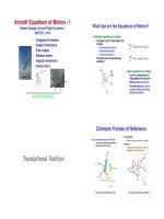
Pitching and Heaving
Wake shape of a
sinusoidally pitching
and heaving airfoil.
Positive vorticity is
denoted by red and
negative by blue

Introduction to Aeroelasticity


Experimental results
Wake vorticity is a realworld phenomenon.
Here is a comparison
between numerical
simulation results (top)
and flow visualization in
a water tunnel (bottom)
by Jones and Platzer.

Introduction to Aeroelasticity


How to model this?
•! The simulation results are useful but

–! Not always accurate (there can be problems
concerning starting vortices for example)
–! Not practical. If the motion (or any of the parameters)
is changed, a new simulation must be performed.

•! Analytical mathematical models of the problem
exist. They were developed in the 1920s and
1930s.
•! Most popular models:
–! Theodorsen
–! Wagner

Introduction to Aeroelasticity


Simplifications
•! In Theodorsen’s approach, only three major
simplifications are assumed:
–! The flow is always attached, i.e. the motion’s
amplitude is small
–! The wing is a flat plate
–! The wake is flat

•! The flat plate assumption is not problematic. In
fact Theodorsen worked on a flat plate with a
control surface (3 d.o.f.s), so asymmetric wings
can also be handled.
•! If the motion is small (first assumption) then the
flat wake assumption has little influence on the
results.
Introduction to Aeroelasticity


Basis of the model
•! The model is based on elementary
solutions of the Laplace equation:
! 2" = 0

•! Such solutions are:
–! The free stream:
–! The source and the sink:
–! The vortex:

–! The doublet:
Introduction to Aeroelasticity

! = U cos"x + U sin "y

"
"
2
2
ln r =
ln ( x $ x 0 ) + ( y $ y 0 )
2#
2#
& y " y0 )
#
#
! = " % = " tan "1 (
+
2$
2$
' x " x0 *
µ cos # µ
x
!=
=
2" r
2" x 2 + y 2
!=

Circle
•! Theodorsen chose to model the wing as a
circle that can be mapped onto a flat plate
through a conformal transformation:

Introduction to Aeroelasticity


Joukowski’s conformal
transformation

•! Define the complex variable z as z=x+iy.
•! Then consider the new complex variable
za, given by:
R2
za = x a + iy a = z +
z
y!

ya!

R!
x!

Introduction to Aeroelasticity

-2R!

2R!

xa!


Singularities
•! Theodorsen chose to use the following
singularities:

–! A free stream of speed U and zero angle of
attack
–! A pattern of sources of strength +2! on the top
and surface of the flat plate, balanced by
sources of strength -2! on the bottom surface
–! A pattern of vortices +"! on the flat plate
balanced by identical but opposite -"!
vortices in the wake

Introduction to Aeroelasticity


y
2!

2!

Complete flowfield
2!
x1,y1

Black dots: sources and sinks
Red dots: vortices

b
+"!

-"!

b2/X0,0

X0,0
x1,-y1

-2!
-2!

Introduction to Aeroelasticity

-2!

The circle radius, b, is equal to
the wing’s half-chord, b=c/2.

x


Complete flowfield – flat
y
plate
Wing
-b

Wake
b

x

Points inside the circle are transformed
outside the flat plate. Therefore, the
vortices inside the circle are mapped on the
wake.
The wing’s chord should have been 4b but
this has been divided by 2 because we are
using sources of strength 2!.
Introduction to Aeroelasticity


About the wing and wake
•! The wing is a flat plate with a source
distribution that changes in time.
•! The +2! and -2! source contributions do
not cancel each other out.
•! The wake of the wing is a flat line with
vorticity that changes both in space and in
time.
•! The +"! and -"! vorticity contributions do
not cancel each other out.
Introduction to Aeroelasticity


Wing and wake are slits
•! Different parts of the circle map to different

parts of the wing
y

Circle upper surface

-b

b
Circle lower surface

Introduction to Aeroelasticity

Outside circle

Inside circle

x


Boundary conditions
•! As with all attached flow aerodynamic
problems there are two boundary
conditions:
–! Impermeability: the flow cannot cross the solid
boundary
–! Kutta condition: the flow must separate at the
trailing edge

•! Kelvin’s theorem must also be observed.
Introduction to Aeroelasticity

Boundary conditions 2
•! The impermeability condition is fulfilled by
the source and sink distribution
•! The Kutta condition is fulfilled by the
vortex distribution
•! Kelvins’ theorem is automatically fulfilled
because for every vortex +"! there is a
countervortex -"! . Therefore, the total
change in vorticity is always zero.
Introduction to Aeroelasticity


Impermeability
•! Impermeability states that the flow normal to
a solid surface is equal to zero.
•! For a moving wing, the velocity induced by
the source distribution normal to the wing’s
surface must be equal to the velocity due to
the wing’s motion and the free stream, i.e.
!"
= #w
!n

•! Where n is a unit vector normal to the surface
and w is the external upwash.
Introduction to Aeroelasticity

Impermeablity (2)
•! Across the solid boundary of a closed
object the source strength is given by
#$
! ="
#n

•! (assuming that the potential of the internal
flow is constant)
•! Therefore, !=w
•! This means that the strength of the source
distribution is defined by the wing’s
motion.
Introduction to Aeroelasticity


Wing motion
•! Assume that the wing has pitch and
plunge degrees of freedom.
•! The total upwash due to its motion is equal
to
˙

(

(

))

w = ! U" + h + b( x1 + 1) ! x f "˙

•! where xf is the position of the flexural axis
and x1 goes from -1 to +1.
x
x=
b

Introduction to Aeroelasticity

and x is measured from the half-chord


Potential induced by sources
•! The potential induced by a source at x1 , y1 is given
by
"
"
2
2
2
2
ln ( x $ x1 ) + ( y $ y1 ) =
ln[( x $ x1 ) + ( y $ y1 ) ]
d! ( x1, y1 ) =
2#
4#

•! By noting that we are using sources of strength 2!,
the potential induced by a source at x1 , y1 and a
sink at x1 , -y1 is given by

2
2
" % ( x $ x1 ) + ( y $ y1 ) (
d! ( x1,± y1 ) =
ln '
*
2# '& ( x $ x1 ) 2 + ( y + y1 ) 2 )*
•! The value of this potential does not change if we
use non-dimensional coordinates
2
2
" % ( x $ x1 ) + ( y $ y1 ) (
d! ( x1,± y1 ) =
ln '
*
2# '& ( x $ x1 ) 2 + ( y + y1 ) 2 *)
Introduction to Aeroelasticity

where x =

x
, y = 1! x 2
b


Total source potential
•! The total potential induced by the sources
and sinks is given by
2
2

%
x $ x1 ) + ( y $ y1 ) (
b
(
! ( x, y ) =
# ln '
2
2 *dx1
+
2" $1
'& ( x $ x1 ) + ( y + y1 ) *)
1

•! Substituting for ! from the upwash
equation we get
2
2
%
x $ x1 ) + ( y $ y1 ) (
b
(
˙
! ( x1, y1 ) =
U# + h + b( x1 + 1) $ x f #˙ ln '
2
2 *dx1
+
2" $1
'& ( x $ x1 ) + ( y + y1 ) *)
1

(

Introduction to Aeroelasticity

(

))


After the integrations
•! A long sequence of hardcore integration
sessions has been censored. Such scenes
are unsuitable for 2nd year Master students
and middle-aged engineering professors.
•! The result on the upper surface is:
2
b
"˙
2
˙
( x + 2) 1# x 2 (1)
! ( x, y ) = b(U" + h # x f "˙ ) 1# x +
2
•! The result on the lower surface is
! ( x, y ) lower = "! ( x, y )
Introduction to Aeroelasticity


Pressure on the surface

•! From the unsteady Bernoulli equation:
% q 2 #$ (
p = ! "' + * + Constant
& 2 #t )

•! Where p is the static pressure, " the air density
and q the local air velocity
•! For calculating the forces on the wing we need to
apply this equation to the wing’s surface.
•! The local velocity on the surface is tangential to
the surface. As the wing lies on the x-axis:
"#
"#
$U +
q = U cos! + u = U cos ! +
"x
"x

Introduction to Aeroelasticity