Vibrations of elastic connecting rod of a high speed slider crank mechanism
Bạn đang xem bản rút gọn của tài liệu. Xem và tải ngay bản đầy đủ của tài liệu tại đây (602.43 KB, 9 trang )
PETER W.JASINSKI
Graduate
Student.
HOCHONGLEE
Adjunct Associate Professor.
Also Employed a t IBM Corp.,
Endicott, N. Y.
Mem. ASME
GEORGE N.SANDOR
A L C O A Foundation Professor
o f Mechanical Design.
Chairman, Division o f
Machines and Structures.
Fellow ASME
Rensselaer Polytechnic Institute,
Troy, N. Y.
Vibrations of Elastic Connecting Rod of a
High-Speed Slider-Crank Mechanism1
The research involved in this paper jails into the area of analytical vibrations applied to
planar mechanical linkages. Specifically, a study of the vibrations, associated with an
elastic connecting-bar for a high-speed slider-crank mechanism, is made. To simplify
the mathematical analysis, the vibrations of an externally viscously damped uniform
elastic connecting bar is taken to be hinged at each end {i.e., the moment and displacement are assumed to vanish at each end). The equations governing the vibrations of the
elastic bar are derived, a small parameter is found, and the solution is developed as an
asymptotic expansion in terms of this small parameter with the aid of the KrylovBogoliubov method of averaging. The elastic stability is studied and the steady-state
solutions for both the longitudinal and transverse vibrations are found.
Introduction
s,
IINCE the kinematics of linkages play an important role in
machine design, research on the subject is extensive. Some investigators considered elasticity or elastic constraints in linkages
[2, 3]2 and others investigated effects of rigid mass inertia
[4-18]. Although a linkage member may have both rigid mass
and flexibility, elasticity and inertia (using harmonic analysis or
graphical methods) have generally been treated separately.
Only for simple mechanisms (such as cam-follower systems) have
combined effects been studied [19, 20]. Since at high speed a
linkage is subjected to its own inertial forces and suffers elastic
deformation, the combined effects must be fully investigated.
Thus, with the speed of machinery constantly increasing, a
detailed mathematical investigation of the vibrations of linkages
is needed. To begin this, one naturally turns to the slider-crank
mechanism which is the simplest linkage (Fig. 1). For the first
step of the mathematical investigation, a model must be chosen
which represents the important characteristics of an actual slidercrank mechanism but which lends itself readily to solvability.
To accomplish this, the elastic connecting bar in Fig. 1 is assumed to be hinged at each end (i.e., the moment and displace-
ments vanish at each end). These boundary conditions are
satisfied exactly by the elastic bar mounted on a rigid slider-crank
mechanism in Fig. 2. These boundary conditions for the connecting bar (displacement and moment being zero at each end)
permit investigation more readily. Thus the model consisting of
a distributed-mass, externally viscously damped elastic bar with
the foregoing boundary conditions is taken as a first approximation for the study of an elastic connecting bar.
But even this simplified model results in a fairly complicated
mathematical representation. The equations governing this
system, in which both longitudinal and transverse vibrations are
considered, are two simultaneous nonlinear periodically time-
1
Based on part of a dissertation by P. W. Jasinski toward fulfillment of the requirements for the Degree of Doctor of Engineering,
Division of Machines and Structures, School of Engineering, Rensselaer
Polytechnic Institute, Troy, N. Y.
2
Numbers in brackets designate References at end of paper.
Contributed by the Design Engineering Division for publication
(without presentation) in the JOUBNAL or ENGINEERING FOB IN-
DTJSTBY. Manuscript received at ASME Headquarters, June 18,
1970. Paper No. 70-DE-C.
Fig. ? M o d e l of a slider-crank linkage with a hinged elastic connecting
bar and a rigid crank
836 / MAY 1 971
Copyright © 1971 by ASME
Transactions of the ASME
Downloaded From: on 09/07/2013 Terms of Use: />
a .
la3. 3
- sm cot —
sm cot
L
6L3
— — sin cot
Letting
X
cot,
il =
L
u
(3)
L
the equations (1) and (2) are written
Fig. 2
Model of a rigid slider-crank linkage w i t h a mounted elastic bar
ITT
+ ( 2 - COS T
vT ~ ( j sm r I v - - — (cos 2r +
AE
variant partial differential equations with periodic forcing functions. These equations are neither readily solvable with the aid
of classical methods nor readily reducible to the well-known
Hill's (or Mathieu) equation. Thus, one is led almost out of
necessity to approximate methods among which the KrylovBogoliubov (K-B for short) asymptotic method of averaging is
foremost. T h e K-B method along with the Galerkin variational
method enables the solution of the above stated problem to be
written in terms of an asymptotic series once a small parameter is
found and the equations are written in standard form [1]. The
nonlinear term is assumed small and disregarded. Also, a small
amount of external viscous damping is assumed.
Introduction of Dimensionless Quantities
pAV-co"1
la2
2 L2
&
p^-co
la2
a
+
-COST
+
- — (COS2T -
city
'dl
—
U
—•
l
+ pA
+
EI
. ,-. v
pAZ/co2 mv
f
a.
a .
+ —r- vr = -V T sm r + - sm r
p^co
L
L
la2
+ - - sm 2r
) •
\ 7~ I +
Reduction to Ordinary Differential Equations
a c 2 G0S
°
(ui ~ 0 )
(1)
vhere
d<t>
(d<t>y
diu'-\'di)
v
+ 2
"
v +
d*<t> - EI
d¥u +
Mv—
T h e displacement and moment are assumed to vanish at each
end of the elastic bar in Fig. 1. The functions sin nirri, where n
is an integer, satisfy these boundary conditions and thus the
Galerkin variational method can be used to reduce the partial
differential equations to ordinary differential equations. Substituting
(T,
+
1
pAA
vt +
(x +
u) —
+
aco cos (cot — <j>)
df
3
( ! ) '
neglected when equations (4) and (5) are written.
pA
d<j>
x
(5)
. . . are small compared with ( - I and f — J and thus can be
Ux
d(f>
tit — v — — aco sili (cot — r/>)
=
(4)
where - has been taken to be
AE
V
dt
1)
( a
\
la2
,
(a .
\
vTT — I 2 — cos T I uT — - — (cos 2r + 1) v + I — sm r 1 u
The system equations, 3 as derived in Appendix 1, are:
V,
l)d
aco2 sin (col — <j>)
7]) = a(r) sin 7rr/, v(r, ij) = j8(r) sin -rij
(6)
into equations (4) and (5), multiplying by sin7nj, and integrating
over t] from 0 to 1, the following is obtained:
(2)
The nonlinear coupling term is disregarded.
a + pi2a = e/i + e2
(7)
/3 + j»22/3 = ifc + 62ff-2
(8)
-Nomenclatureu =•• longitudinal vibration (in.)
v = transverse vibration (in.)
u = dimensionless longitudinal vibration
v = dimensionless transverse vibration
t = real time (sec)
T = dimensionless time
L = length of elastic bar (in.)
a = length of crank (in.)
a; = spatial coordinate for elastic
bar (in.)
1} — dimensionless spatial coordinate
r/> = angle defined in Fig. 1
co = angular velocity of crank
(l./sec)
E = Young's modulus (psi)
I = area moment of inertia about
neutral axis (in. 4 )
A = cross-sectional area (in. 2 )
p = mass density (lb-sec 2 )/in. 4
, p 2 2 = dimensionless natural frequencies
a = dimensionless
longitudinal
first mode
/? = dimensionless transverse first
mode
t = dimensionless small parameter
^) / = proportionality constants for
e, f —
cii, (h,} _
hi, h2 )
Si, cii, \ _
bi, h )
>, < =
», «
=
= =
—• =
== =
viscous damping (lb-sec/
in. 2 )
dimensionless proportionality
constants
new dimensionless dependent
variables
new dimensionless dependent
variables as given by second
approx.
"is greater than," "is less
than"
"is much greater t h a n , " "is
much less t h a n "
"equal by definition"
"approaches"
"almost equal t o "
Journal of Engineering for Industry
Downloaded From: on 09/07/2013 Terms of Use: />
MAY 1 971 / 637
where
Vi
+ ( - Pa + - j &2 sin (p2 +
AEir*
pA L2co2'
=
EIT*
X 62 sin (p 2 — pi -
/i = - cos T — 2/3 cos r + /3 sin r
(9b)
ir
1
1
3
ai = - a cos 2 T -\— a -\— cos 2 r
2
7T
1
ea
sin (p t - 1) T +
(9d)
X 61 sin (pi - p 2 + 1 ) T Af
(9e)
and the parameters are chosen to satisfy
e
f IJ
/ = - ^ - - !2 = 1
pAu a
+
4/
„))) + - H i sin (pi + p 2 + 1) T
hl Ssin
i
(p, — p a — 1) r +
" ^ ' ~ P 2 ~~ ^ T + \ 2
X 62 cos (pi — p 2 — 1) r — I 'z Pi + ^ ) *>2
(9/)
ai(r), ai(r), 6i(r), b 2 (r)
A3 =
defined bj r the relations,
a = ai sin pir + a2 cos p i r
(106)
(3 = hi sin p 2 r + 62 cos p 2 r
(10c)
/3 = pin cos j)2r — p262 sin p2T
(lOd)
2
+
G»-i)- )ai cos (p
\2
Vl +
4/
+
° ^
( 2 Pi + A a"-
(e/i + f2(/i) sin pir
sin
(He)
{efi + e2<72) sin pir
X4 =
(Hd)
Pi
+
The equations (11) are in the form
x = eX(x,r) + « 2 Y(X,T)
(12)
1
- cos (p2 — 1 ) T
1 )r
'
~ \2
xt
~ 4/
Ft
F2
F3
F,
Pl
~ 4)
(13c)
G-0
cos (p s + 1 ) T
11
!
ai sin (p 2 + pi - 1 ) T + I - pi - + ^ a , sin
, (p 2 + pi + 1 ) T
l
2Pl
+ I - Pi + - j ai sin (p 2 - pi - 1 ) T
y ^
Pl
1
X ai sin (p2 - pi + 1 ) T + (I 2- ^
where 4
+
1
4
X ch cos (P2 — pi — l ) r + I - pi + - ja 2 cos (p 2 + pi + 1 ) T
and
_
2
2
- cos (pi — 1 ) T H— cos (pi + 1 ) T
ir
COS (pi — p 2 + 1) T
( 2 V, - 4 ) 61 co,
+
X a2 sin (p t — p 2 — 1 )r
P2
Pi
'
(Pi + Vi + D r - f -
(116)
61 = — (e/ 2 + e2a2) cos p 2 r
ir
P
( - pi + - J a2 sin (pi - p 2 +
Pi
A'i
(\
1
- pi + l ) r + I - pi - -
2
ai C S
sin (pi -f- p 2 - 1 ) T -
Pi
X3
(136)
(11a)
di = — (e/i + e ai) oos pir
rx2 i
1^
cos (p 2 + Pi - l ) r + ( - Pi + - J »i cos (p 2 - pi -
are introduced into equations (7) and (8), the following equations
result:
X 4
(P1 + Vi + 1) T
1 .
1
- - sin (p 2 — l ) r H— sm (p 2 + l ) r
T
ir
P2
+
(10a)
a = pidi cos p i r — pia 2 sin pLr
xi
4/
X 62 cos (pi 4- p 2 — 1 ) T
If four new unknown dependent variables,
62 = —
cos
P2 +
'1
62 cos (p, - p 2 + 1) r - l - p 2
Reduction to Standard Form
d2 =
sin (pi + 1 ) T
f 2 P2 ~ 4 ) fei s i l 1 (Pi + P2 ~ 1)^ "" ( 2 ^ 2 ~ 4 )
-
\ 2 V'2
e V
= — - 2 * 1,
pAu a
l)r
pi L I T
(9c)
7T
2
1 T2
Xt =
2
fi — - sin r + 2 d cos r — a sin r
ir
a
e = - « 1,
L
{Cont.)
(9a)
pALW
2
(13a)
+ 1 ) T + ( - Pi - - j
Pl
/I
\2
Pl
1\
~ 4 j * ° 0 S P'2
_
Pl +
1 )r +
-
/l
1
Vi Pl ~ 4
X a2 cos (p 2 + pi — 1 ) T
-G-0
F,
Pi
(13d)
1
3
3
- a2 + — cos (pj + 2 ) T + —- cos (pi - 2)r
4
27r
2ir
X 61 cos (p, + p 2 — l ) r — ( - p 2 + - j 61 cos (pi - p 2 — 1 ) T
-
2
( - P + ^ J &i cos (pi + p 2 + l ) r + ( - Pi - - J
X 62 sin (p s + pi — l ) r + ( - p 2 + - j 62 sin (p2 — p, + 1 ) T
4
It is understood that terms like cos (pu — T) are written as cos
(pi - 1) r.
638 / M A Y 1 9 / 1
- - cos pit + - Oi sin (2pi + 2)r + - 01 sin (2px — 2)r
7T
8
8
+ - a2 cos (2pi + 2 ) T + - a2 cos (2pi — 2 ) T + - o2 cos 2 r
8
8
4
1
.
1
+ - ai sin 2 pir H— a2 cos 2pir
4
4
1
•
eai cos 2pir
2
1
1
-eai + ~ (Mi sm 2piT
(14a)
Transactions of the AS ME
Downloaded From: on 09/07/2013 Terms of Use: />
1
3
3
- fd + — siii (pi + 2)r + —- sin (pj - 2 ) T
Yi
4
M
2ir
2TT
1 . 1
1
— - sin piT — - ai cos (2p! + 2)r — - ai cos (2px — 2)r
7T
8
1
8
.
where
1
+ - a2 sin (2pi + 2)r + - a2 sin (2pi — 2)r + - ai cos 2r
8
8
4
1
1
.
1
— - ai cos 2piT + - a2 sm 2j>iT + - eai sin 2p t r
4
(17)
[V]
Vi = J(pu p 2 )a 2 + K(pi, p 2 ) cos (pi — 2)r
1
4
M
**)*]*
T
Z
1
^i
ea2
+ - ecii cos 2p1T
(146)
+ B(pi, p2)d2 cos (2jh - 2)r
7 2 = -J"(pi, p 2 )a, + E(plt p2)di cos (2pi - 2)r
(18b)
F 3 = / ( p 2 , pi)Su + I?(p2, Pi)S2 cos (2p 2 — 2 ) T
(18c)
1^4 = —J{.Pi, Pi)Si — 27f(p2, Pi) cos (p2 -
2)r
+ E{pi, pi)b, cos (2p 2 - 2 ) T
1
Y3 = - - 62 H
4
P'2
1
1
sin (p2 4- 2)r — - sin (p2 — 2)r
7T
where
+ - 63 cos 2p 2 r — - fbi cos 2 p 2 r
2 ^
J(y, 2)
1
1
1
+ 2)r 4- - b2 cos (2p2 — 2)r + - 62 cos 2r 4- - 6i sin 2p 2 r
8
4
4
+
4
y - z 4- 1
i-i
?/ + 2 + 1
+
IT
IC(?/, «) =
bi cos (2p2 — 2)r + 8
8
8
,N
fbi + - / 6 2 sin 2p 2 r
TV
bi cos (2p 2 4- 2)r
4
(ly+i)(l°-\
1
1
1
- bi H— cos (p2 — 2)r — - cos (p2 4- 2)r
Pi
Z
4/ \2
2/ + 2 - 1
(14c)
Yt
(18d)
5
7T
1
1
1
+ - 6, sin (2?;2 4- 2 ) T + - 6i sin (2p 2 - 2)r + - 62 cos (2p,
o
8
8
(18a)
yz
1
1
-2 + 12
4
4A2
E(y, z) =
2/2
1
.
1
bi cos 2p2T + - b2 sin 2 p 2 r -\— fbi sin 2p2T
4
4
2'
(196)
^4
y+ z - 1
2V
+
(14d)
1
-Z - 12
4
7T Z 4 - 1
1
— - /6 2 + - /6 2 cos 2 piT
1
r + —r~r
1 2 - 1
X b2 sin (2p 2 + 2 ) T + - 62 sin (2p2 - 2 ) T 4- - 6, cos 2r
8
4
(19a)
y - z - 1
1\ / l
l) \2
1
Z
'
y - 2 - 1
(19c)
I t should be noted that only those terms which can potentially
contribute to — [V] are included in equations (18).
The Method of Averaging the Second Approximation
The equations (11) being in the form (12) are seen to be in
standard form for application of the K-B method of averaging
[1]. As indicated in Appendix 2, the second approximation is
governed b}' the equations,
^ ^
[ X ] + £
T
^
^
[ y ] + £
T
T
x «p) x'
(15)
where for a vector function F(x,r) in the form
F ( x , r ) = 2 Fc(x)
e
ex
P i®T
Also, the
T
(16a)
terms (19) are written for the most general case in t h a t the denominators were assumed not to vanish. For those cases in
which they do vanish, the terms with vanishing denominators
are simply disregarded as indicated in equation (16c). Thus there
is no possibility of division by zero.
Examining equations (13), (14), (18), it is seen that equations
(15) must be considered separately for cases which correspond to
different points in the pit p 2 plane. The four major cases now
follow and it should be remembered throughout that 0 < e « 1,
e = 1 , / = 1, p ! > 0 , p 2 > 0 .
Case 1. Consider all (pi, p 2 ) which satisfy pi 5^ 1, 2; p 2 9^ 1, 2;
p 2 5^ pi ± 1, p 2 j£ — pi 4- 1. Equations (15) are written as
with the 6 being constant frequencies,
M
-
[F(x,r)] 4 F„(x)
F(x,r) = E
F» (x)
exp idr
fli = e2fi(pi, pi)&2 — - e2cai
(20a)
d, = — e2fi(pi, p 2 )ai — - e2ea2
(20b)
bi = e2Q(p2, pi)b 2 — - e2/6i
(20c)
b2 = — e2fl(p2, pi)bi — - e2/62
(20d)
(16b)
(16c)
0^0
M.
The operator — is known as the averaging operator and ~ as the
r
integrating operator. The vector ^ is written here as
~d,
P=
where
^2
_6 2 _
From equations (13),
fi(2/, 2) = J(y, 2) +
Mi
Equations (20) are easily uncoupled and it is seen that the solu6
y and 2 are "dummy variables."
Journal of Engineering for Industry
Downloaded From: on 09/07/2013 Terms of Use: />
MAY 1 97 1 / 639
tions are asymptotically stable in that di, di, Si, bi -* 0 as r -*• oo,
independent of initial conditions.
Case 2.
Consider all (pi, p2) which satisfy p 2 = Pi — 1 and
p 2 5^ 1, 2. Equations (15) become
1
1
2P2
&x =
+
i
eSi
?2 + 1
+
) —^—
_4p 2
+ 1
+ H(V,_ + 1, p2)
Thus, as in Case 1,
&i, d%, b\, 62 ->• 0 as
1
1
2Pl
+
2
Q2
=
P2 +
i
Pi + 1
1
— - ee2Oi
i —J— + H{Vi + l, p2)
= 52 -
e 2 di
1
+
i
61 =
«oi +
1
1
2
di =
eb2
_4p.
Pi
•:
.4p5
+ 7(p2 + 1, p2)
62b2
;/e'6i
-2 P2
+
+ I(pi + 1, pi)
(21c)
1
1
~ Pi -\—
2
4 „
61 = Pi +r~T~
1 «°i +
„
—
p2
+ /(P2 + 1, Pi)
e 2 b,
1
_*P2
,
; /e 2 b 2
l_4 Pi + *
(26b)
--/e«fci
(26c)
J
(21d)
62 =
1
2 P l+ i
- 4 - r + #(Pi + 1. Pi)I e26i
Pi + 1
J
—7 ten —
Pi + 1
- /t s b 2
where
-G"-i-)G--0
H(», 0 = ^
d\, di, bi, hi —» 0 as r —»• 00
v+
(i i)6*~i) G^M^J)
+
1/ + z + 1
z — 2/ — 1
(22a)
Case 4. Consider all (pi, p 2 ): which satisfy p2 =
Equations (15) are written for this case as
1
.
Hv,*)-
"2 i)(l'-Q
y -
P
' - i .
ebi +
Pi
z + 1
— + A(p„ - p , + 1)
1
y+z- 1
1
di =
-
2
"i
.
— + A(Pl, -vi + 1)
.4pi
Pi
(24)
61 =
The roots of the algebraic equation (24) are called characteristic
values. If the real parts of all characteristic values are negative,
the solution is asymptotically stable. This is shown with the
aid of Routh's stability criterion [21] which states that the characteristic values all have negative real parts if
(25a)
ai(a3a2 — a4ai) —
a32a0
> 0
e'ai
- ee2d2
where Z is a matrix defined by the equivalence of equations (21)
with (23). The characteristic equation of the system (21) is seen
to be6
«o, ai, a2, a3, a* > 0
2Pl
4
tdi
1 - Pi
+
1
1
.4 1 - Pi
+ A (-p, + ],Pl)
(276)
e2b2
- - / f 2 6 , (27c)
1
bi =
1
2^24
" 1 - P i
1
€0 2 —
1
_4 1 — pi
+ A(-Pl
+ 1, p,)
e26i
(25b)
-2/e2b
6
det is short for d e t e r m i n a n t a n d I is used here as t h e i d e n t i t y
matrix.
640 / M A Y 1 9 7 1
(27a)
1
P l
ebi
(23)
Z) = a,X4 + a3X3 + a2X2 + oA + a0 = 0.
ee2d\
(226)
Equations (21) are in the form
det(XI -
ezo2
.4pi
y
C -i)(i'-j)
—pi + 1.
1
2
di =
y+z+ i
y+
(26d)
These equations are very similar to those of case 2 and it is
similarty seen, using Routh's criterion, that
y+ «— l
yz
+
- e^d,
[~7 - 4 - : + H(Pl + 1, pi)"|
1
4
(26a)
_4 p 2 + 1
, 1
2P2
1
+ /(Pi + 1, Pi)
Pi
1
•
A
4 ,
ebi +
di =
ee di (21a)
1
-*• co.
Case 3. Consider all (pi, p2) which satisfy p 2 = pi + 1 and
pi ^ 1, 2. Equations (15) are for this case
e2a2
2
T
2
(27d)
where
Transactions of the ASME
Downloaded From: on 09/07/2013 Terms of Use: />
2
A(\),z)
„,
OG-i)
- JV +
= —
yz
x +1
+ e2
2 +
—
—
y+ «+ l
/ s m ( p i + 2)r
Pa) (
T^
V
Pi + 2
IT
c o s ( p i + 2)T
Q(pi, P2)
PI + 2
_i
cos (p 2 +
(28)
y+ l
sm(pi-2)r\
^T~ ) +
p, - 2
/
cos(pi — 2 ) r \
)+
Pi - 2
/
h
Q(PK
4
2Q(P2, P.)
2)T
+
Pi + 2
2Q(P2, Pi)
COS piT
(p 2 —
Pi
2)T
)
p2 — 2
sin (p 2 — 2)'
p2 + 2
! = ££
s piT
sin
' P2^
Pi
S(p1,P2)
COS
sin(p2 + 2 ) T
as in cases 2 a n d 3, t h e e q u a t i o n s (27) a r e in t h e f o r m
S(Pl
-')
P2
with a characteristic equation
.
(30)
(Cont.)
a 4 X 4 + a 3 X 3 + a 2 X 2 + aiX + ao = 0
B u t u n l i k e cases 2 a n d 3, R o u t h ' s s t a b i l i t y c r i t e r i o n ( i n e q u a l i t i e s
(25)) is n o t satisfied for all v a l u e s of pi, e, e, f. B u t a d i g i t a l c o m p u t e r m a y b e u s e d t o i n v e s t i g a t e t h e s e i n e q u a l i t i e s for t h i s case.
I t is f o u n d
t h a t t h e r e is a n i n t e r v a l c e n t e r e d
G3
at
w h e r e x 8S is t h e s t e a d y - s t a t e s o l u t i o n a n d
t
for
w h i c h t h e s o l u t i o n s of (27) a r e a s y m p t o t i c a l l y s t a b l e . B u t a t
t h e e n d r e g i o n s of t h e line s e g m e n t p 2 — —pj + 1, p i > 0, p% >
0, e l a s t i c i n s t a b i l i t y e x i s t s a n d t h e s o l u t i o n g r o w s e x p o n e n t i a l l y .
If t h e v i s c o u s d a m p i n g is i n c r e a s e d , t h e l e n g t h of t h e s t a b l e
region is i n c r e a s e d . T h u s , a l t h o u g h it is possible to effectively
remove t h e elastic instability b y m a k i n g t h e viscous d a m p i n g
l a r g e e n o u g h , case 4 f u r n i s h e s t h e o n l y p o s s i b i l i t y for i t s p r e s e n c e .
Additional Cases
T h e lines pi, p 2 = 1, 2 h a v e b e e n e x c l u d e d from t h e p r e v i o u s
four cases a n d m u s t b e c o n s i d e r e d s e p a r a t e l y . W h e n t h i s is d o n e ,
they are found to be elastically stable and correspond t o b o u n d e d
s o l u t i o n s of t h e s y s t e m ( 1 5 ) .
Q(v, 2)
x = I + 6X +
+ e 2 (x
e>9
w h e r e ^ satisfies e q u a t i o n s (15).
^ )
X -
d
e"
(29)
X„
*
&*
Letting r
2 sin (pi
ill
2 sin (pi +
1)T
X
1)
x
1)
(30)
(Ji
02
pi(pi
2 cos (pi
l)r
2 cos (pi -f-
1)T
X
1)
X
1)
Pi(pi
1 COS (p 2
61
pi(pi +
X
p-lipi
Pl(pi +
1 cos (p 2 +
• Dr
— 1)
7T
1 sin (p-i — l ) r
X
3
2TT
sin (pi 4- 2 ) r
Pl(p,
+
_3_ cos ( p t +
+ e2
2x
p-l(Pi
2)
+ „~
2x
pi(pt
cos (pi
+' 2 x
2)
2)r
pi(pi — 2)
1 cos (p 2 +
2)r
1 cos (p 2
•r
2)
x
p2(p2 +
1 sin (p 2 — 2 ) r
x
p2(p2 -
2)
p2(p2 -
1 sin (p 2 +
x
p 2 (p 2 +
=
1
1
- «+ -
4
2 +
X 7/2
a"
(r) = e
2 1
1
1
- z —2
1
4
Z -
(32)
1
1
x pi \ p i — 1
L.27TP1
+
pi +
1
1
+ <3(Pl, P2)
/3»»(T)
=
+ a'
e
_1 1_
1
x p2
- 1
e
1_
+• p
+ pi
Pi + 2
1
+ t
1
x piz
-
2T
a
+ S(pu p2) - I (33a)
pi.
1
+ 2Q(p 2 , p i )
h]°°cosf
+ 1
2
1
+
_Vi + 2
,7T p 2
sin
2T
(33b)
p2
Examination of the Steady-State Solutions
T h e extent to which the approximate steady-state solutions
(33) s a t i s f y t h e e q u a t i o n s (7) a n d (8) is easily f o u n d . W r i t i n g all
of t h e t e r m s i n (7) a n d (8) o n t h e l e f t - h a n d s i d e a n d s u b s t i t u t i n g
(33), t h e e r r o r r e s u l t s o n t h e r i g h t - h a n d s i d e :
, (Z
pi2 - p22
4^ \ X (p! 2 - l ) ( p 2 2 -
5pi 2 — p 2 2 — 16
1
D(P2 2 - ~ 4 )
cos
3T
\
, /
4e
1 \ .
1
COS T + I —
) Bill T
2
4)/
\
TT Pi - 1 /
J
l)r
p 2 ( p 2 4- 1)
sin (pi — 2 ) r
2)T
pi(pi + 2)
T
1
2
(31)
1
x (p> -
1)
1 sin (p 2 +
1)
2 + 1
a + p i 2 a — e/i — e2
l)r
p 2 (p2 +
x yz
l
2* + 4
T h e s t e a d y - s t a t e first m o d e s for b o t h t h e l o n g i t u d i n a l a n d t r a n s verse vibrations m a y now be found using equations (10a) a n d
(10c).
The Improved Second Approximation and the Steady-State
Solutions
A s p r e v i o u s l y s h o w n , for cases 1, 2, 3 ( w h i c h b e s i d e s s o m e
o t h e r p o i n t s e n c o m p a s s t h e p o i n t s pi > 2, p 2 > 2 ) t h e s e c o n d a p p r o x i m a t i o n s o l u t i o n s di, m, hi, b-i a p p r o a c h zero w i t h i n c r e a s i n g
d i m e n s i o n l e s s t i m e T . T h u s it is n o t a difficult t a s k t o e x a m i n e
t h e s t e a d y - s t a t e s o l u t i o n s of t h e i m p r o v e d s e c o n d a p p r o x i m a t i o n
for t h e s e cases. A s s e e n i n A p p e n d i x 2, t h e i m p r o v e d s e c o n d a p p r o x i m a t i o n x is g i v e n b y
z)
l
i*"i
2 ^
S(y,
i
1 1_
P22 -
+ 64
4 x (p,
1 sin p ^
pi2
x
1 cos p i r
x
•2)r
pi2
2
x pi (p,
2)
2)r
2)
-
(pi 2 2
+ (-?
-
2
2
(p, 2 -
2
4)(p22 -
1)(P2 2 -
Pa'
4)(p22 -
+
4 x pi (pi
1)
1)
(p 2 2 2
4T
2)
4)(p,2 -
2
cos
1)
cos
sin
2)(pi2 — 4)(p2
Journal of Engineering for Industry
Downloaded From: on 09/07/2013 Terms of Use: />
2
2T
2T
s:
~)
(34a)
MAY 1 97 1 / 641
2
Pi /3 - «/, - e2!72
a«s —» 0 as — if pi —• <*> (or u —»• 0)
"/l
15p22 - p! 2 - 26 \ .
/2/
1
\
sin ST + (
c
e>
_\27T (pi 2 - 4)(p 2 2 - 1)7
\7T p 2 2 - 1 /
9p 2 2 - pi 2 - 14
( 1
^
V27T (pi 2 - 4)(p 2 2 - 1)
+ e4
p22 - 2
1
j3" —>• 0 as —
if p 2 -»- co (or co -*- 0)
p22
.
7T P!2(P22 - 1 ) /
2
[/ 1
\
Pi2
- Pi + 4
\ . ,
1—
sin 4r
_\27r (vi1 - l)(p 2 2 - 4 ) 7
, /1
" Vi% + 4
\
\TT (p, 2 - l)(p 2 2 - 4 ) /
. „
T
pi 2 - 4
/4/
\
+ u (P1.-i)(P,.-4);co82Tj
(346)
As expected, the error only contains e to t h e third and higher
orders. For pi, p 2 S> 2 and 0 < e « 1, the error is seen to be small
and thus the approximate steady-state solutions (33) satisfy the
equations (7) and (8) very well. But the error is unbounded near
Pi, Pi — 0, 1, 2 and thus the validity of (33) is questionable near
these values. Furthermore, examining Appendix 3, where the
averaging method is applied to an equation in which the exact
solution is known, more light is shed on this. T h e equation in
Appendix 3 contains a sinusoidal forcing function with a frequency X. Comparing the approximate solution (by the averaging method) to the exact solution, it is seen t h a t the approximate
solution is very good for large X b u t veiy poor for small X. In
fact the approximate solution is unbounded for small X where the
exact solution is bounded for small X. So if X is restricted to be
large ( \ » « ) , the method of averaging works well. Similarly, the
solutions (33) should be restricted to pi, p 2 5>> 2 and it should not
be concluded that a", (3" are unbounded for pi, p 2 = 0, 1, 2.
The Final Result
If pi, p 2 » 2, Q(p 1; p 2 ), Q(p2, pi), S(pi, p^ may be neglected in
equations (33) which may be written:
a" (at)
cos cot 4- e2 I - —
) cos 2ut
2
\ T Pi I
IT
pi
+ \
T Pi-1
(3SS (fat) = e (
) sin cot +e
\ T Pi
\ T P227
/4
= t I
1 \
, n
I L sm — COS OJ<
2
\7T p i /
L
7TX
\7T P i 2 /
/
L sin — cos 2 coi + e2 I
L
\
1
IT
1 \
1TX
) L sin — (36a)
pi2/
L
, N
,2 l \ r
. n .
v"(x, t) — € [
r I L sin — sm oil
\7T p 2 2 /
L
+ 6;
(*L)
\TT p 2 2 7
Li
Conclusion
It has been shown that a, /3, may be written as
P = (3"-»"» + ft"
trana
where the transient terms a
, (3
approach zero with increasing T and the steady-state terms a", (3" are periodic in t
27T
with period
642 / MAY
Also,
197 1
increasing the viscous damping.
For higher approximations than t h e second, many more cases
need be considered (i.e., pi, p 2 = integers), but these added cases
will not affect t h e stability results since t h e signs of the critical
terms in t h e stability analysis are dominated by t h e e and eterms. Also, in higher approximations, additional constant forcing terms appear (as they did for pi, p 2 = 1, 2) but they will be of
the order of e" for the nth approximation. Thus additional terms
will appear in t h e steady-state solutions obtained from t h e improved n t b -approximation b u t they will affect the one derived
here onty slightly (i.e., with terms of e3 and higher).
The foregoing results were obtained with some restrictions and
assumptions. Hinged end conditions were assumed at each end
(i.e., t h e moment and displacements were assumed to vanish at
each end). T h e nonlinear coupling term was assumed to be
small and was dropped. A small amount of external viscous
damping was assumed (that is, e, f = 1). Finally, t h e dimensionless parameter e was chosen small relative to 1.
This paper has demonstrated the value of the K-B method of
averaging for the study of the dynamics of linkages. Future work
in this area m a y include attempts to determine the elastic
stability of higher-order linkages using similar asymptotic methods. Also, it may be possible to perform a more sophisticated
analysis on the slider-crank mechanism. This analysis may determine the effect of the nonlinear coupling term and may involve
more suitable boundary conditions such as a free-end condition or
an end with a concentrated mass present.
Acknowledgment
Support under N S F Grant No. GK-4049 awarded to Rensselaer Polytechnic Institute in response to a proposal submitted
by the second and third authors and sponsored by the Engineering
Mechanics Program, Engineering Division of t h e National
Science Foundation, is greatly appreciated. The authors would
also like to express their appreciation to Mrs. Frances K. Willson
for typing t h e manuscript and to Mrs. Diane Jasinski for her
computer programming aid.
References
L sin 2oii sin — (366)
where pi, p 2 S> 2.
tranB
Pi = Pi = - • The length of the stable region may be increased by
sin 2 cot (35b)
where T has been replaced by u>l. Using equations (3), (6), (35),
the steady-state longitudinal and transverse vibrations become
x,t)
That is, the vibrations have small amplitudes for small rotating
speeds.
The only possibility of elastic instability occurs on the line
segment p 2 = — pi + 1, pi > 0, p 2 > 0. The regions of instability
and stability here are determined by Routh's stability criterion
which leads to complicated inequalities which depend upon pi, e,
e, f. The instability regions are restricted to the end regions of the
line segment and the stability region is centered at t h e point
1 Bogoliubov-Mitropolsky, Asymptotic Methods in the Theory
of Nonlinear Oscillations, Gordon and Breach, New York, 1961.
2 Burns, R. H., "Kinetostatic Synthesis and Analysis of Flexible
Link Mechanisms," Doctoral Dissertation, Yale University, September 1964.
3 Livermore, D. F., "The Determination of Equilibrium Configurations of Spring-Restrained Mechanisms Using (4 X 4) Matrix
Methods," JOURNAL OF ENGINEERING FOR INDUSTRY, TRANS. ASME.
Series B, Vol. 89, No. 1, Feb. 1967, pp. 87-93.
4 Chace, M. A., "Analysis of the Time-Dependence of MultiFreedom Mechanical Systems in Relative Coordinates," JOURNAL OF
ENGINEERING FOR INDUSTRY, TRANS. ASME, Series B, Vol. 89, No. 1,
Feb. 1967, pp. 119-125.
5 Crossley, F . R. E., "The Balancing of High-Speed Oscillating
Feed Mechanisms," ASME Paper No. 64-Mech-28.
6 Han, Chi-Yeh, "Balancing of High Speed Machinery,"
JOURNAL OF ENGINEERING FOR INDUSTRY, TRANS. ASME, Series B,
Vol. 89, No. 1, Feb. 1967, pp. 111-118.
Transactions of the ASME
Downloaded From: on 09/07/2013 Terms of Use: />
7 Uicker, J. J., Jr., " D y n a m i c Force Analysis of Spatial L i n k ages," Journal of Applied Mechanics, Vol. 34, T H A N S . A S M E , Series
E, Vol. 89, 1967, N o . 2, p p . 418-424.
8 Beyer, R . A., " S t a t i c s and D y n a m i c s in 3-D M e c h a n i s m s , "
Transactions of the Sixth Conference on Mechanisms, October 1 0 - 1 1 ,
1960, p p . 94-11.2.
9 Sieber, H . , "Analytische u n d graphische Verfahren zur S t a t i k
und D y n a m i k raumlicher Kurbelgetriebe," Z. Konstruktion,
1959,
pp. 333-344.
10 Root, R. E., Dynamics of Engine and Shaft, J. Wiley & Sons,
1932.
11 Biezeno, C. B., and G r a m m e l , R., Engineering
Dynamics,
Vol. 4, Blackie & Son, London, 1954.
12 Freudenstein, F . , " H a r m o n i c Analysis of C r a n k - a n d - R o c k e r
M e c h a n i s m s with Applications," Journal of Applied
Mechanics,
Vol. 26, T B A N S . A S M E , Series E , Vol. 8 1 , N o . 4, D e c . 1959, p p .
673-675.
13 Yang, A. T., " H a r m o n i c Analysis of Spherical F o u r - B a r
M e c h a n i s m s , " Journal of Applied Mechanics, Vol. 29, T R A N S . A S M E ,
Series E, Vol. 84, N o . 4, D e c . 1962, p p . 683-688.
14 R a n k e s , H . , " H a r m o n i c s Analyse und M a s s - S y n t h e s e , "
Konstruktion, N o . 1,1960, p p . 8-10.
15 M e y e r zur Capellen, W., " K i n e m a t i k u n d D y n a m i k der K u b e l shleife," Werkstatt & Betrieb, N o . 1, P a r t 1,1956, p p . 581-584.
16 M e y e r zur Capellen, W., "Zeichnerisch-rechnerische E r m i t t lung von Massenkraften in K u r b e l t r i e b e n , " Konstruktion,
Vol. 14,
1962, N o . 6, p p . 227-233.
17 M e y e r zur Capellen, W., and D i t t r i c h , G., "Zeichnerischrechnerische von Kraften in Gelenkgetrieben," Ind.-Anz.,
Vol. 83,
No. 84, 1961, p p . 1583-1586 and Vol. 84, N o . 13, 1962, p p . 2 0 9 - 2 1 1 .
18 M e y e r zur Capellen, W., and Dittrich, G., " D i e Energieverteilung in K u r b e l t - r i e b e n , " Z. Feinwerktechnik,
Vol. 64, N o . 6, 1960,
pp. 195-199.
19 K n i g h t , B . A., "Vibration Analysis of Flexible Cam-Follower
S y s t e m s , " M a s t e r ' s Dissertation, Georgia I n s t i t u t e of Technology,
M a r . 1965.
20 Cesari, Asymptotic
Behavior and Stability
Problem in Ordinary Differential Equations. 2, Auflage Springer, Berlin, 1963.
21 T o u , J. T., Digital and Sampled-Data Control Systems, M c G r a w Hill, 1959.
22 H o u s n e r - H u d s o n , Applied
Mechanics—Dynamics,
D . Van
N o s t r a n d , Inc., 1959, p . 40.
23 Meirovitch, Analytical
Methods in Vibrations,
Macmillan,
1967.
APPENDIX
T h e force a n d m o m e n t e q u a t i o n s for t h e differential e l e m e n t
( c e n t e r e d a t x) a r e n o w w r i t t e n in t h e classical w a y [ 2 3 ] :
P H
Q -\
dx — Q — fVi
M + — dxdx
w h e r e pAdx
(pAdx)ax
dx =
(pAdx)a„
(39)
M + Qdx -
Pvx dx = 0
= m a s s of t h e differential e l e m e n t ,
P =
AEux
M =
BIvxx
Vt
(40)
= au cos (ul — d>) + Vi + (x + u)
d<j>
—
dt
and t h e r o t a t o r y inertia and shear deformation are neglected.
E x t e r n a l v i s c o u s d a m p i n g is a s s u m e d in t h e x a n d y - d i r e c t i o n s .
S i m p l i f y i n g (39) a n d u s i n g t h e q u a n t i t i e s i n (38), (40) t h e
equations are derived:
utt
— 2
d4
d2c£
/d<t>y
AE
ft — I — - ) u — TV2 " ~ ~~,T u**
\ dt J
dt
pA
dt
e
pA
r
\u,
d(j)
=
i
_ „ - _ « , , sin (ut -<t>)j
f.dd>y
+ x
{ - )
2
+ aco cos '(ut — </>)
vt, + 2
d<j>
dt
pA I
-. +
\ dt J
d*d>
TTTT l H
df-
+
(41a)
EI
7 "x
pA
AE ,
dip
(x + u) — -4- au cos (oil — <j>) H
7 (v.xVx)x
dt
pA
h au2 sin (ut — d>)
— x
(416)
df
w h e r e ( M A ) , is a n o n l i n e a r c o u p l i n g t e r m .
J + 2"xi (37)
d2p
—
d.c
Ut = — aio s i n (ut — <j>) + ut — V
dt
1
T h e d e r i v a t i o n b e g i n s w i t h t h e w e l l - k n o w n r e s u l t f r o m dynamics [22]:
a = A+coX(
dx — P — iUtdx
dx
Derivation of the System Equations
dut
+ — X 9
at
dP
dx
do
APPENDIX
2
where
a = a c c e l e r a t i o n s e e n from fixed c o o r d i n a t e s y s t e m
A = a c c e l e r a t i o n of m o v i n g c o o r d i n a t e s y s t e m
to = a n g u l a r v e l o c i t y of m o v i n g c o o r d i n a t e s y s t e m
p ~ p o s i t i o n v e c t o r for p a r t i c l e in m o v i n g c o o r d i n a t e s y s t e m .
T h e a c c e l e r a t i o n of a differential e l e m e n t of t h e e l a s t i c b a r in
F i g . 1 m a y b e d e t e r m i n e d u s i n g (37) w i t h
A
=
The Method of Averaging
S u p p o s e t h a t a n a p p r o x i m a t e s o l u t i o n is d e s i r e d for t h e s y s t e m
of differential e q u a t i o n s 7
x = eX(x, r ) + 6 2 Y(x, r )
w h e r e X, Y a r e i n t h e f o r m of F defined b y
—aa) 2 [cos(ui — <j>)\ + sin (coi — 4>)W
F(x, r ) = £
p = (x + u)\ + v),
d'p
dp
— = v,\ +
dt
F,(x) exp
(idr)
vt\
a n d t h e 6 a r e c o n s t a n t f r e q u e n c i e s a n d 0 ' < e
T h u s a = ax\ + atJ) h a s b e e n d e t e r m i n e d w h e r e
,
=
utt
Define t h e
d
r
ax
(42)
2
TtVl
(d
M
(43o)
d?4
(x + u) I — I - v
A2
— aw 2 cos (not — (j>)
e x p idr
(38a)
F = E F<
(43b)
d*4>
d<j>
Cty = Vi, + 2 — Ut
at
[F] = F„
by
dt
v + (x + u) df
aw 2 sin (OJ« -
0)
(386)
7
All q u a n t i t i e s are dimensionless
Journal of Engineering for Industry
Downloaded From: on 09/07/2013 Terms of Use: />
MAY 1 97 1 / 643
T h e Krylov-Bogoliubbv (K-B for short) method of averaging [1]
gives
APPENDIX
3
Examination of the Method of Averaging
= £ + ex + e
!
x
*+-( 4) --*h
(44)
x = — ex — e sin Xr
as an approximate solution where <; is defined by
^^[X1+^i[y]+^[(xJ
T
T
T 1_\
)*]
(45)
Oi;
these coefficients are large (of the order - or larger), the error is
large and the approximation (44) is poor.
644 / M A Y 19 7 1
(46)
The method of averaging gives the approximate solution
The solution to (45) is known as the second approximation and
(44) as the improved second approximation. The approximate
solution (44) satisfies (42) to the order of e3; t h a t is, if (44) is substituted into (42), and (45) is considered, the error only involves
terms containing e3 and higher. Thus, if the coefficients of e3,
e4, . . . in this error are of the order of 1 or less, the error is seen to
be small and the approximation solution (44) is good. But if
€
Consider the differential equation
cos
x = c exp ( —er) + e •
where c is an arbitrary constant.
unbounded in X for small X.
T h e exact solution to (46) is
(47)
This approximate solution is
eX
x — c exp ( — er) H—; , ^~ cos
+ X*
AT
XT
e2
€ + X^2, sin Xr
2—'
(48)
which is bounded in X for small X. Comparing the exact solution
(48) with the approximate solution (47), the method of averaging
is seen to work very well for large X but very poorly for small X
Transactions of the ASME
Downloaded From: on 09/07/2013 Terms of Use: />