Hafez a radi, john o rasmussen auth principles of physics for scientists and engineers 03

34

2 Vectors

(2) A car travels 6 km due east and then 4 km in a direction 120◦ north of east. Use
both the graphical and analytical methods to find the magnitude and direction
of the car’s displacement vector.
→

(3) Vector A has a magnitude of 10 units and makes 60◦ with the positive x-axis.
→
Vector B has a magnitude of 5 units and is directed along the negative x-axis.
→
→
Use geometry to find: (a) the vector sum A + B , and (b) the vector difference
→
→
A − B.
(4) A car travels in a circular path of radius 10 m. (a) If the car traveled one half of
the circle, find the magnitude of the displacement vector and find how far the
car traveled. (b) Answer part (a) if the car makes one complete revolution.

Section 2.3 Vector Components and Unit Vectors
→

→

(5) Vector A has x and y components of 4 cm and −5 cm, respectively. Vector B
→
→
→

has x and y components of −2 cm and 1 cm, respectively. If A − B + 3 C = 0,
→
then what are the components of C .
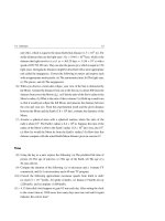
(6) Three vectors are oriented as shown in Fig. 2.15, where A = 10, B = 20, and
→

→

C = 15 units. Find: (a) the x and y components of the resultant vector D = A +
→
→
B + C , (b) the magnitude and direction of the resultant vector.
Fig. 2.15 See Exercise (6)

y

B
C

30

o

30

o

x

A

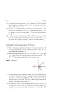
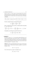
(7) The radar beam of a police car points at an angle of 30◦ away from the direction
of a highway. The radar records the component of the car’s speed along the
beam as vCR = 120 km/h, see Fig. 2.16. (a) What is the speed vC of the car
along the highway? (b) Can the radar beam be directed perpendicular to the
direction of the highway? Why or why not?
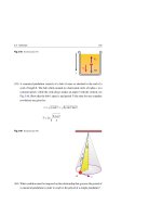
(8) A radar device detects a rocket approaching directly from east due west. At
one instant, the rocket was observed 10 km away and making an angle of 30◦
above the horizon. At another instant the rocket was observed at an angle of 150◦


2.5 Exercises

35

in the vertical east-west plane while the rocket was 8 km away, see Fig. 2.17.
Find the displacement of the rocket during the period of observation.

CR

30

o

C

m
ea

Car velocity

rb

a
ad

R
Police car

Fig. 2.16 See Exercise (7)

Ro c ke t
8k

m

10

150°

km

30°

W

E

Radar Dish

Fig. 2.17 See Exercise (8)

→

→

(9) Find the vector components of the sum R of the displacement vectors A
→
and B whose components along three perpendicular directions are Ax = 2,
→

Ay = 1, Az = 3, Bx = 1, By = 4, and Bz = 2. Find the magnitude of R.
→
→
(10) Two vectors A and B (of lengths A and B, respectively) make an angle θ
with each other when they are placed tail to tail, see Fig. 2.18. (a) By taking
components along two perpendicular axes, prove that the length of their vector
→
→
→
sum R = A + B is:
R=
→

→

A2 + B2 + 2AB cos θ
→

(b) For the difference C = A − B , where C is the length of the third side of a
→
→

triangle formed from connecting the head of B to the head of A as in Fig. 2.19,
use the same approach to prove that:


36

2 Vectors

C=

A2 + B2 − 2AB cos θ

Fig. 2.18 See Exercise (10)

y

R
B

θ

x
A

Fig. 2.19 See Exercise (10)

y

C

B
θ

x
A
→

→

→

(11) A position vector →
r = x i + y j + z k makes angles α, β, and γ with the
x, y, and z axes of a perpendicular right-handed coordinate system as in
Fig. 2.20. Show that the relation between what is known as the direction cosines
cos α, cos β, and cos γ are as follows: cos2 α + cos2 β + cos2 γ = 1.
Fig. 2.20 See Exercise (11)

z

r
γ
α

y

x
→

→

→

→

β

z

y
x

→

(12) When vector B is added to vector A we get 5 i − j , and when B is sub→
→
→
→
tracted from A we get i − 7 j . What is the magnitude and direction of A ?


2.5 Exercises

37
→

→

→

→

→

→

(13) Two vectors are given by A = 2 i + 3 j and B = 4 i − 3 j . Find: (a) the
→ →
→
magnitude and direction of the vector sum R = A + B , (b) the magnitude and
→ →
→
direction of the vector difference S = A − B .
→ →
→
→
→ →
→
→
(14) Two vectors are given by A = − i + j + 4 k and B = 3 i − 4 j + k . Find:
→
→
→
→
→
→
→
→
(a) A + B , (b) A − B , and (c) a vector C such that A + B + C = 0.

Section 2.4 Multiplying Vectors
→

(15) Vector A has a magnitude of 3 units and lies along the negative x-axis. Vector
→
B has a magnitude of 6 units and makes an angle 30◦ with the positive x-axis.
→ →
(a) Find the scalar product A • B without using the concept of components.
→ →
(b) Find A • B by using vector components.
→

→

→

→

→

(16) Show that for any vector A : (a) A • A = A2 and (b) A × A = 0.
→
→
(17) In Exercise 10, show that dotting vector R with itself and dotting vector C
with itself leads directly to the results of both part (a) and part (b).
→ →
→ →
(18) For the vectors in Fig. 2.21, find the following: (a) A • B , (b) A • C ,
→
→

→ →
→ →
→
→
(c) B • C , (d) A × B , (e) A × C , and (f) B × C .
Fig. 2.21 See Exercise (18)

y

C

4 B

5

x

3

A
→

→

→

→

→

(19) (a) Show that A • (A × B ) = 0 for all vectors A and B . (b) If θ is the angle
→
→
→
→ →
between A and B , then find the magnitude of A × (A × B ).
→
→
(20) Two vectors A and B make an acute angle θ with each other when they are
placed tail to tail as shown in Fig. 2.22. (a) Prove that the area of the triangle
→ →
that is contained by these two vectors is 21 | A × B |. (b) Show that the area of
→

→

→

→

the parallelogram formed by A and B is | A × B |.
→
→ →
(21) Show that A • (B × C ) is equal in magnitude to the volume of the paral→ →

→

lelepiped whose sides are formed from the three vectors A , B , and C as shown
in Fig. 2.23.

38

2 Vectors

Fig. 2.22 See Exercise (20)

B

θ
A
Fig. 2.23 See Exercise (21)

B

A

C

(22) In the xy plane, point P has coordinates (x1 , y1 ) and is described by the posi→
→
tion vector →
r 1 = x1 i + y1 j . Similarly, point Q has coordinates (x2 , y2 )
→
→
and is described by the position vector →
r 2 = x2 i + y2 j , see Fig. 2.24.
→
(a) Show that the displacement vector from P to Q is given by d = →
r2 −→

r1 =
→

→

→

(x2 − x1 ) i + (y2 − y1 ) j . (b) Find the magnitude and direction of d .
Fig. 2.24 See Exercise (22)

y

Q( x2 , y2 )

r2

d
P(x1 ,y 1 )

r1

o
→

→

x

→

(23) The equation F = q(v→ × B ) gives the force F on an electric point charge q
→
moving with velocity v→ through a uniform magnetic field B. Find the force on
→
→
a proton of q = 1.6 × 10−19 coulomb moving with velocity v→ = (2 i + 3 j +
→
→
4 k ) × 105 m/s in a magnetic field of 0.5 k tesla. (The given SI units yield a
force in newtons.)
→
→
→
→
(24) The electromagnetic Poynting vector S is defined by S = E × H , where
→
→
→
→
→
E and H are the electric and magnetic fields. Calculate S for E = i +
→
→
→
→ →
→
0.3 j + 0.5 k and H = −0.4 i + j + 0.2 k. You can disregard units for this
calculation.

Part II

Mechanics


3

Motion in One Dimension

Mechanics is the science that deals with motion of objects. It is basic to all other
branches of physics. The branch of mechanics that describes the motion of objects
is called kinematics. In this branch we answer questions like “Does the object speed
up, slow down, stop, or reverse direction?” and “How is time involved in these
situations?”
In this chapter, we only study motion along straight lines. The moving object of
concern is either a particle (a point-like object) or an object that can be viewed to
move like a particle.

3.1

Position and Displacement

To locate an object in one-dimensional space, we find its position with respect to
some reference point, called the origin of an axis, such as the x-axis shown in Fig. 3.1.
The positive/negative direction of this axis is the direction of increasing/decreasing
numbers.
A change in the object’s position from an initial position xi to a final position xf
is called displacement x (read delta x), where:
Negative direction
Positive direction

x
-3

-2

-1

0

1

2

3

Fig. 3.1 The position of a particle that moves in one dimension is identified on an x-axis that is marked
in units of length

H. A. Radi and J. O. Rasmussen, Principles of Physics,
Undergraduate Lecture Notes in Physics, DOI: 10.1007/978-3-642-23026-4_3,
© Springer-Verlag Berlin Heidelberg 2013

41


42

3 Motion in One Dimension

x = xf − xi

(3.1)

The displacement is a vector quantity which has a magnitude and a direction. The
magnitude is the distance between the initial and final positions and the direction is
represented in Fig. 3.1 by a plus or minus sign for motion to the right or to the left,
respectively.

3.2

Average Velocity and Average Speed

Average Velocity
Consider a particle moving along the x-axis, where its position-time graph is as
shown in Fig. 3.2. At point P, let its position be xi when the time was ti and at point
Q, let its position be xf when the time was tf (the indices i and f refer to the initial
and final values for the variables under consideration). Accordingly, during the time
interval t = tf − ti , the particle’s displacement is x = xf − xi .
x

Q

xf
Slope =

Δx
P

Δt

xi
O

ti

tf

t

Fig. 3.2 The position-time graph for a particle moving along the x-axis. The slope of the line PQ measures
the average velocity v

One of several quantities associated with the phrase “how fast” a particle moves
is the average velocity, v, which is defined as follows:
Average velocity
The average velocity, v, of a particle is defined as the ratio of its displacement,
x, to the time interval, t. That is:


3.2 Average Velocity and Average Speed

v=

43

x
xf − xi
=
t

tf − ti

(3.2)

From this definition, v has the dimension of length divided by time, that is m/s
in SI units. The average velocity is a vector quantity which has a magnitude and
direction represented by a plus or minus sign for motion to the right or to the left,
respectively, see Fig. 3.1.

Average Speed
The average speed s is a different way of describing “how fast” a particle moves and
it is defined as follows:
Average speed
The average speed, s, of a particle is defined as the ratio of the total distance
covered d to the time interval t = tf − ti . That is:

s=

total distance
d
=
t
tf − t i

(3.3)

So, s is different from v in that s does not depend on direction, and hence is always
positive. In some cases s might be the same as v.
Example 3.1

A car moving along the x-axis starts from the position xi = 2 m when ti = 0 and
stops at xf = − 3 m when tf = 2 s. (a) Find the displacement, the average velocity,
and the average speed during this interval of time. (b) If the car goes backward
and takes 3 s to reach the starting point, then repeat part (a) for the whole time
interval.
Solution: (a) The car’s displacement, see Fig. 3.3, is given by:
x = xf − xi = −3 m − 2 m = −5 m
The average velocity is then given by:
v=

x
−3 m − 2 m
xf − xi
−5 m
=
=
=
= −2.5 m/s
t
tf − ti
2s−0s
2s


44

3 Motion in One Dimension

Since

x and v are negative for this time interval, then the car has moved to

the left, toward decreasing values of x, see Fig. 3.3. The total covered distance is
d = 5 m and the average speed is thus:
s=

d
5m
total distance
5m
=
=
= 2.5 m/s
=
t
tf − ti
2s−0s
2s

In this case, s is the same as v (except for a minus sign).
tf=2s

ti=0
Negative direction

|

|

|

|

|

|

-3

-2

-1

0

1

2

x (m)

Fig. 3.3 Example 3.1

(b) After the backward movement, the final position and final time of the car
are xf = 2 m and tf = 2 s + 3 s = 5 s, respectively, while the total distance
covered by the car is d = 5 m + 5 m = 10 m. As we know, the displacement
involves only the initial and final positions and will be:
x = xf − xi = 2 m − 2 m = 0
Then, the average velocity will be:
v=

x
0
xf − xi
=
=
=0
t
tf − ti
5s−0s

Finally, the average speed for the whole movement of the car will be:
s=

d
10 m
total distance
10 m
=
=
= 2 m/s
=
t
tf − ti
5s−0s
5s

As you can see, the average velocity is zero, while the average speed is 2 m/s,
since the latter depends only on the total covered distance d.

3.3

Instantaneous Velocity and Speed

More commonly, we ask how fast a particle is moving at a given instant, which
refers to its instantaneous velocity (or simply velocity). The velocity at any instant
is obtained from the average velocity by allowing the time interval t to approach
zero. Consider the motion of an object (for example a car). This object can be viewed


3.3 Instantaneous Velocity and Speed

45

as a particle for simplicity. The motion of that particle between two points P and
Q on a position-time graph is shown in the right part of Fig. 3.4. As point Q is
brought closer and closer to point P (through points Q1 , Q2 , . . .), the time intervals
( t1 , t2 , . . .) get progressively smaller. The average velocity for each time interval
is the slope of the dotted line in Fig. 3.4. As point Q approaches P, the time interval
approaches zero, while the slope of the dotted line approaches the slope of the tangent
to the curve at point P. This slope is defined to be the instantaneous velocity v at the
time ti . In short, we define:
Instantaneous velocity
The instantaneous velocity, v, of a particle is defined as the limiting value of the
ratio

t approaches zero. Mathematically v can be expressed as:

x/ t as

v = lim

t→0

x
t

(3.4)

x

ti

Q2

tf

P
Δ t2

xi
o
xi

P

Q

Q1

Slope of the tangent =

x

o

Q2 Q1 Q

ti

Δ t1

Δt

tf

t

Fig. 3.4 The left part shows a police car (which can be considered as a particle) that moves along the
x-axis. The right part shows the position-time graph for this motion. As Q approaches P, the average
velocity v for the interval PQ approaches the slope of the tangent line at P, which is defined as the
instantaneous velocity v at point P

In calculus notation, the above limit is called the derivative of x with respect to t, and
written as dx/dt (abbreviated as x˙ ). Thus:
v=

dx
dt

≡

xf − xi =

tf
ti

v dt ≡ Area under v-t graph

(3.5)


46

3 Motion in One Dimension

The instantaneous velocity, v, can be positive, negative, or zero, depending on the
slope of the position-time graph at the interval of interest in Fig. 3.5. In this figure,
v = 0 represents the turning point, and occurs at any maximum or minimum of the
x-t graph. From here on, we use the word velocity to denote instantaneous velocity.
The speed of a particle is defined as the magnitude of its velocity.

x

Inflection points

0

t

t1

t2

Fig. 3.5 The position-time graph for a particle moving along the x-axis. On this graph we display:
(1) Positive velocities, where the slope of the tangent lines are positive, (2) Negative velocities, where the
slope of the tangent lines are negative, (3) Zero velocities (turning points), where the slope of the tangent
lines are zero, and (4) Inflection points at t1 and t2 , where the increase/decrease of the velocity reaches a
maximum/minimum

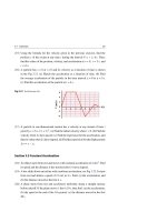
Example 3.2

A particle moves along the x-axis and its coordinates vary with time according
to the relation x = t 2 − 2 t, where x is measured in meters and t is in seconds.
The position-time graph for this motion is shown in Fig. 3.6. (a) Use this graph to
comment about the particle’s motion. (b) Find the displacement and the average
velocity of the particle in the time intervals 0 ≤ t ≤ 1 s and 1 s ≤ t ≤ 3 s.
(c) Find the velocity of the particle at t = 2 s.
Solution: (a) The particle starts from the origin of the x-axis and moves in the
negative x direction for the first second. Its velocity is zero at x = −1 m when
t = 1 s and then heads back in the positive x direction for t > 1 s.
(b) In the interval 0 ≤ t ≤ 1 s we have ti = 0 and tf = 1 s. Since x = t 2 − 2 t,
we get xi = ti2 − 2 ti = 0 and xf = tf2 − 2 tf = −1 m. Thus:
x = xf − xi = −1 m − 0 m = −1 m


3.3 Instantaneous Velocity and Speed
Fig. 3.6

47

x(m)

3

Slope = 2

2

1
Slope = −1
t(s)

0
1

2

3

-1

The average velocity is then:
v=

xf − xi
−1 m
x
−1 m − 0 m
=
=

= −1 m/s
=
t
tf − ti
1s−0s
1s

According to Fig. 3.6, this value equals the slope of the straight line drawn for
this time interval.
In the interval 1 s ≤ t ≤ 3 s we have ti = 1 s and tf = 3 s. Again, from x =
2
t − 2 t we get xi = ti2 − 2 ti = −1 m and xf = tf2 − 2 tf = 3 m. Thus:
x = xf − xi = 3 m − (−1 m) = 4 m
The average velocity is then:
v=

xf − xi
4m
x
3 m − (−1 m)
=
=
= 2 m/s
=
t
tf − ti
3s−1s
2s

According to Fig. 3.6, this value equals the slope of the straight line drawn for

this time interval.
(c) To find the instantaneous velocity at any time t, we use Eq. 3.5 and apply
the rules of differential calculus on the coordinate x = t 2 − 2 t. That is:
v=

d(t 2 − 2t)
dx
=
= 2t − 2
dt
dt


48

3 Motion in One Dimension

Notice that this expression gives the velocity v at any time t and indicates that v
is increasing linearly with time. It tells us that v < 0 during the interval 0 ≤ t < 1 s
(i.e. the particle is moving in the negative x direction), and that v = 0 at t = 1 s,
and finally v > 0 for t > 1 s. When t = 2 s we use the above expression to get:
v = 2 × 2 − 2 = 2 m/s

3.4

Acceleration

When the velocity of a particle changes with time, the particle is said to be accelerating. Consider the motion of a particle along the x-axis. If the particle has a velocity
vi at time ti and a velocity vf at time tf as in the velocity-time graph of Fig. 3.7, then
we define the average acceleration as:

Average acceleration
The average acceleration, a, of a particle is defined as the ratio of the change
in velocity v = vf − vi to the time interval t = tf − ti . That is:

vf − vi
v
=
t
tf − ti

a=

(3.6)

Q
f
a=

Δ
Δt

P
=

ti

P

i

=

tf

Q

i

f

x

0

Δ
Δt

ti

tf

Fig. 3.7 The velocity-time graph for a car (or simply a particle) moving in a straight line. The slope of
the straight line PQ is defined as the average acceleration in the time interval

t = tf − ti


3.4 Acceleration

49

Acceleration is a vector quantity having dimensions of length divided by (time)2 , or
L/T2 ; that is m/s2 in SI units.
It is useful to define the instantaneous acceleration as the limit of the average
acceleration when t approaches zero. Consider the motion of a particle (for example
a car that moves like a particle) between the two points P and Q on the velocitytime graph shown in the right part of Fig. 3.8. As point Q is brought closer and
closer to point P (through points Q1 , Q2 , . . .), the time intervals ( t1 , t2 , . . .) get
progressively smaller. The average acceleration for each time interval is the slope of
the dotted line in Fig. 3.8. As Q approaches P, the time interval approaches zero, while
the slope of the dotted line approaches the slope of the tangent to the curve at point
P. The slope of the tangent line to the curve at P is defined to be the instantaneous
acceleration a at the time ti . That is, we define the following:
Instantaneous acceleration
The instantaneous acceleration, a, of a particle is defined as the limiting
value of the ratio
be expressed as:

v/ t when

t approaches zero. Mathematically a can

a = lim

(3.7)

Q

a

t→0

v
t

nt =

Q1

Slo
pe o

f ta

nge

Q2

=

ti
P

=

i

tf

Q2

Q1

Q

P

i

f

x

0

Δt 2
Δ t1

ti

t2

Δt

t1

tf

t

Fig. 3.8 The left part shows a car that moves along the x-axis. The right part shows the velocity-time

graph that describes the car’s motion. As Q approaches P, the average acceleration a for the interval
PQ approaches the slope of the tangent line at P, which is defined as the instantaneous acceleration a at
point P


50

3 Motion in One Dimension

In calculus notation, the above limit is called the first derivative of v with respect
to t, and written as dv/dt (simplified sometimes as v),
˙ or the second derivative of x
2
2
with respect to t, and written as d x/dt (simplified sometimes as x¨ ). Thus:
a=

dv
d2x
= 2
dt
dt

≡

vf − vi =

tf

a dt ≡ Area under a-t graph

(3.8)

ti

From here on, we use the word acceleration to designate instantaneous acceleration. Depending on the slope of the tangent to the velocity-time graph, acceleration
a can be positive, negative (called deceleration), or zero. If a = 0 for a specific time
interval in the v − t graph, then the velocity must be a constant in this interval.
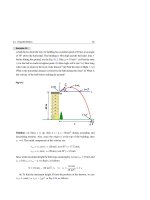
Example 3.3

The position of a particle moving along the x-axis varies with time t according to
the relation x = t 3 − 12 t + 20, where x is given in meters and t in seconds. (a)
Find the velocity and the acceleration of the particle as a function of time. (b) Is
there ever a time when v = 0? (c) Describe the particle’s motion for t ≥ 0.
Solution: (a) To get the velocity v as a function of time t, we differentiate the
coordinate x with respect to t as follows:
v=

d 3
dx
=
t − 12 t + 20
dt
dt

⇒

v = 3 t 2 − 12

To get the acceleration a as a function of time t, we differentiate the velocity v

with respect to t as follows:
a=

d
dv
=
3 t 2 − 12
dt
dt

⇒

a = 6t

(b) Setting v = 0 in the velocity relation yields:
0 = 3 t 2 − 12,
which has the solution t = ±2 s. The negative answer has to be rejected, since
time must be always positive. Thus at t = 2 s the velocity of the particle is zero.
(c) To describe the particle’s motion for t ≥ 0 we examine the expressions
x = t 3 − 12 t + 20, v = 3 t 2 − 12, and a = 6 t.
At t = 0, the particle is at x = 20 m from the origin and moving to the left
with velocity v = −12 m/s and not accelerating since a = 0, see Fig. 3.9.


3.4 Acceleration

51

At 0 < t < 2 s, the particle continues to move to the left (x decreases), but at a
decreasing speed, because it is now accelerating to the right, a = positive (Check

the expressions of x, v, and a for t = 1 s and compare the results with Fig. 3.9).
At t = 2 s, the particle stops momentarily (v = 0) to reverse its direction of
motion. At this moment x = 4 m, i.e. it will be as close as it will ever be to the
origin. It will continue to accelerate to the right at an increasing rate, see Fig. 3.9.
For t > 2 s, the particle continues to accelerate and move to the right, and its
velocity, which is now to the right, increases rapidly, see Fig. 3.9.
Fig. 3.9

x (m)
25
Left motion

20

Right motion

15
10
5

t (s)

0
0

1

2

3

1

2

3

(m /s)
20
10

t (s)

0
-10

0

-20

a (m /s 2 )
20
15
10
5

t (s)

0
0

1

X Data

2

3


52

3.5

3 Motion in One Dimension

Constant Acceleration

In many common types of one-dimensional motion, the acceleration is constant (or
we say uniform). In this case, the average acceleration equals the instantaneous
acceleration, i.e.
a = a = constant

(3.9)

The shape of this relation can be displayed for positive a as shown in the left part of
Fig. 3.10. Consequently, Eq. 3.6 becomes:
a=

vf − vi

(when a = a = constant)
tf − ti

(3.10)

Fig. 3.10 (Left part) The acceleration-time graph of a particle moving along the x-axis with constant
acceleration. (Middle part) the velocity-time graph of the particle’s motion. (Right part) The position-time
graph of the particle’s motion

For convenience, we let ti = 0 and tf = t, where t is any arbitrary time. Also, we let
vi = v◦ (the initial velocity at time t = 0) and vf = v (the velocity at any time t).
With this notation, we can express acceleration as:
a=

v − v◦
t

Rearranging gives:
v = v◦ + a t

(for constant a)

(3.11)

This linear relationship enables us to find the velocity at any time t; see the middle
part of Fig. 3.10.
We can make use of the fact that when the acceleration is constant (i.e. when the
velocity varies linearly with time according to Eq. 3.11 as in Fig. 3.10), the average

3.5 Constant Acceleration

53

velocity in any time interval is the arithmetic mean of the initial velocity, v◦ , and the
final velocity at the end of that interval, v. Thus:
v=

v◦ + v
2

(for constant a)

(3.12)

To find the displacement as a function of time, we first let xi = x◦ (the initial position
at time t = 0) and xf = x (the position at any time t), and then use Eq. 3.2 and Eq. 3.12
to get:
v=

v◦ + v
x − x◦
=
t
2

Rearranging gives:
x − x◦ = 21 (v◦ + v) t

(for constant a)

(3.13)

We can obtain another useful expression for the displacement by substituting Eq. 3.11
into Eq. 3.13 to get:
x − x◦ = v◦ t +

1
2

(for constant a)

a t2

(3.14)

As a first check for Eq. 3.14, one can notice that substituting t = 0 yields x = x◦ ,
as it must be. A further check, taking the derivative of Eq. 3.14 with respect to time,
yields Eq. 3.11. The right part of Fig. 3.10 displays the position x as a function of
time t for the parabolic Eq. 3.14.
We can use Eq. 3.11 to eliminate v◦ from Eq. 3.14 to obtain the following relation:
x − x◦ = v t −

1
2

a t2

(for constant a)

(3.15)

Finally, by replacing the value of t that was obtained from Eq. 3.11 into Eq. 3.13, we
can obtain an expression that does not include the time variable as follows:
x − x◦ = 21 (v◦ + v)

(v 2 − v◦2 )
(v − v◦ )
=
a
2a

Rearranging gives:
v 2 = v◦2 + 2 a (x − x◦ )

(for constant a)

(3.16)

Equations 3.11 through 3.16 are six kinematic expressions used to solve any onedimensional problem with constant acceleration.
Table 3.1 lists the four kinematic equations that are used most often in solving
problems for the case of constant acceleration.


54

3 Motion in One Dimension

Table 3.1 Equations for motion with constant acceleration
Equation

Missing quantity

Equation number

v = v◦ + a t

x − x◦

Eq. 3.11

x − x◦ = 21 (v◦ + v) t

a

Eq. 3.13

x − x◦ = v◦ t +

t2

v

Eq. 3.14

v 2 = v◦2 + 2 a (x − x◦ )

t

Eq. 3.16

1
2

a

Example 3.4

A car accelerates uniformly from rest to a speed of 100 km/h in 18 s.(a) Find the
acceleration of the car. (b) Find the distance that the car travels. (c) If the car
brakes to a full stop over a distance of 100 m, then find its uniform deceleration.
Solution: (a) In this problem we are given v◦ = 0, v = 100 km/h, and t =
18 s = 5 × 10−3 h and we need to find a. So, we can use v = v◦ + a t to find
the acceleration as follows:
a=

100 km/h − 0
v − v◦
1,000 m
= 2 × 104 km/h2 ≡ 2 × 104
=
= 1.54 m/s2
−3
t
5 × 10 h
(60 × 60 s)2

(b) If the car starts from the origin of the x-axis, i.e. x◦ = 0, then we are given

v◦ = 0, v = 100 km/h, x◦ = 0, and t = 5 × 10−3 h and we need to find x, which in

this case equals the distance traveled by the car. So, we use x − x◦ = 21 (v◦ + v) t
to find the position x as follows:
x = x◦ + 21 (v◦ + v) t = 0 + 21 (0 + 100 km/h) × 5 × 10−3 h = 0.25 km = 250 m

(c) We are given v◦ = 100 km/h, v = 0, and x − x◦ = 0.1 km and we need to
find the deceleration a. We use v 2 = v◦2 + 2 a (x − x◦ ) to get:
a=

v 2 − v◦2
0 − (100 km/h)2
=
= −5 × 104 km/h2 = −3.86 m/s2
2 (x − x◦ )
2 × 0.1 km

Example 3.5

In a cathode ray tube of a TV set, an electron with initial velocity v◦ = 2 × 104 m/s
enters a region 2 cm long (see Fig. 3.11) where it is electrically accelerated in a
straight line. The electron emerges from this region with a velocity v = 3×105 m/s.
(a) What was its acceleration, assuming it was constant? (b) How long will the
electron be in this region?


3.5 Constant Acceleration

55

Fig. 3.11

2cm

Solution: (a) Taking the motion to be along the x-axis, and using v◦ = 2 ×

104 m/s, v = 3 × 105 m/s, and x − x◦ = 2 cm = 2 × 10−2 m, we can find the acceleration a from the relation v 2 = v◦2 + 2 a (x − x◦ ) as follows:
a=

(3 × 105 m/s)2 − (2 × 104 m/s)2
v 2 − v◦2
=
= 2.24 × 1012 m/s2
2 (x − x◦ )
2 × 2 × 10−2 m

(b) Since the displacement and velocities are known, we can use x − x◦ =
1
2 (v◦

+ v) t to find the time t that the electron will be electrically accelerated as
follows:
t=

2(x − x◦ )
2 × 2 × 10−2 m
=
= 1.25 × 10−7 s = 0.125 µs
v◦ + v
2 × 104 m/s + 3 × 105 m/s

Another way to find t is to use equation v = v◦ +a t. In this case, v = 3×105 m/s,

and a = 2.24 × 1012 m/s2 . Thus:
t=

v − v◦
3 × 105 m/s − 2 × 104 m/s
= 1.25 × 10−7 s = 0.125 µs
=
a
2.24 × 1012 m/s2

Even though a is very high in this example, but such an acceleration occurs
over a very short time interval which is a typical value for such an electrically
accelerated charged particle.

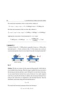
∗Example 3.6

The remote-controlled truck shown in Fig. 3.12 moves along the x-axis with a
constant acceleration of −2 m/s2 . As it passes the origin, i.e. x◦ = 0, its initial
velocity is 14 m/s. (a) At what time t and position x does v = 0 (i.e. when the


56

3 Motion in One Dimension

truck stops momentarily)? (b) At what times t1 and t2 is the truck at x = 24 m,
and what is its velocity then?
t1 , 1

t 0 , ° 14 m/s

2 m/s 2

a

2 m/s 2

a

t,

0

2 m/s 2

a

x
x 24m

x

0

t2 , 2

2 m/s 2

a

x
x 24m

0
Fig. 3.12

Solution: (a) Given v◦ = 14 m/s, v = 0, and a = −2 m/s2 , we can find t by
using v = v◦ + a t as follows:
t =

v − v◦
0 − 14 m/s
=7s
=
a
−2 m/s2

To find the position x we can use v 2 = v◦2 + 2 a (x − x◦ ), since we are given
v◦ = 14 m/s, v = 0, x◦ = 0, and a = −2 m/s2 . Thus:
x = x◦ +

v

− v◦2
0 − (14 m/s)2
=0+
= 49 m
2a
2 × (−2 m/s2 )

2

(b) Using x = 24 m, x◦ = 0, v◦ = 14 m/s, and a = − 2 m/s2 in x − x◦ = v◦ t +
1
2

a t 2 , we find, after omitting the units temporarily, that:
24 − 0 = 14 t +

1
2

(−2) t 2

⇒

t 2 − 14 t + 24 = 0

Solving this quadratic equation yields:
t=

14 ±

(−14)2 − 4 × 1 × 24
14 ± 10
=
2×1
2

⇒

t=

t1 = 2 s
t2 = 12 s

Thus, t1 = 2 s is the time the truck takes from the origin to the position x = 24 m.
Furthermore, t2 = 12 s is the time the truck takes from O, passing the point
x = 24 m, reaching the point x = 49 m and returning back to x = 24 m.


3.5 Constant Acceleration

57

For x = 24 m, v◦ = 14 m/s, a = −2 m/s2 , and t1 = 2 s, we use the formula
v = v◦ + a t to get v1 as follows:
v1 = v◦ + a t1 = 14 m/s + (−2 m/s2 ) × (2 s) = 10 m/s
Also, for x = 24 m, v◦ = 14 m/s, a = −2 m/s2 , and t2 = 12 s, we use the
formula v = v◦ + a t to get v2 as follows:
v2 = v◦ + a t2 = 14 m/s + (−2 m/s2 ) × (12 s) = −10 m/s
Observe that the two speeds are equal, i.e. |v1 | = |v2 | = 10 m/s.
In this example, we do not pay any attention to the cause of this constant
acceleration, but this will be clarified later on when we study the dynamical
aspect of mechanics.

3.6

Free Fall

Due to gravity, it is well known that all dropped objects near the Earth’s surface
will accelerate downward with a nearly constant acceleration when the effect of air
resistance is very small and can be neglected. We use the term “free fall” for this
motion and the same will be applied to objects that are either thrown up or down.
We shall denote the magnitude of the acceleration due to gravity by the symbol g,
which is very close to 9.8 m/s2 near the Earth’s surface.
Therefore, for free falls near the Earth’s surface, the constant acceleration equations of motion Eqs. 3.11 through 3.16, and hence equations of Table 3.1, can be
applied. However, we can make them simpler to use with the following minor
changes:
(1) The motion is along the vertical y-axis.
(2) The free-fall acceleration is negative if the y-axis is chosen to be upward, and
hence we replace the acceleration a with −g.
(3) The free-fall acceleration is positive if the y-axis is chosen to be downward, and
hence we replace the acceleration a with +g.
Table 3.2 lists the four kinematic equations that are frequently used in solving
free-fall problems with constant acceleration, where always |a| = g = 9.8 m/s2 for
motions near the Earth’s surface.


58

3 Motion in One Dimension

Table 3.2 Equations for free-fall motion with constant acceleration
y (up), a = −g

Equation

y (down), a = g

y↑

v = v◦ − g t

y↓

Equation
v = v◦ + g t

y − y◦ = 12 (v◦ + v) t

y − y◦ = 21 (v◦ + v) t

y − y ◦ = v◦ t −

y − y◦ = v◦ t +

v2

=

v◦2

1
2

g t2

v2

− 2 g(y − y◦ )

=

v◦2

1
2

g t2

+ 2 g(y − y◦ )

Example 3.7

A ball is dropped from a tall building, as shown in Fig. 3.13. Choose the positive
y to be downward with its origin at the top of the building, i.e. y◦ = 0. Find the
following for the ball’s motion: (a) its acceleration, (b) the distance it falls in 2 s,
(c) its velocity after falling 15 m, (d) the time it takes to fall 25 m, and (e) the time
it takes to reach a velocity of 29.4 m/s.

y

Fig. 3.13

≈

≈
y

Solution: (a) Since the positive y is downward, then the ball’s acceleration is
positive (downward) and will be given by a = g = 9.8 m/s2 . Also, the ball’s
velocity will be always positive.
(b) We are given v◦ = 0, y◦ = 0, a = g = 9.8 m/s2 , and t = 2 s. To find y,
we use y − y◦ = v◦ t + 21 g t 2 as follows:
y=0+

1
2

(9.8 m/s2 ) × (2 s)2 = 19.6 m

(c) We are given v◦ = 0, y◦ = 0, a = g = 9.8 m/s2 , and y = 15 m. To find
v, we use v 2 = v◦2 + 2 g(y − y◦ ) as follows:
v 2 = 0 + 2 × (9.8 m/s2 ) × 15 m

⇒

√
v = ± 294 m/s

⇒

v = 17.2 m/s

(d) We are given v◦ = 0, y◦ = 0, y = 25 m, and a = g = 9.8 m/s2 . To find
t, we use y − y◦ = v◦ t + 21 g t 2 as follows:
25 = 0 + 21 (9.8 m/s2 ) × t 2

⇒

√
t = ± 5.1 s

⇒

t = 2.3 s


3.6 Free Fall

59

(e) We are given v◦ = 0, v = 29.4 m/s, and a = g = 9.8 m/s2 . To find t, we
use v = v◦ + g t as follows:
t=

v − v◦
29.4 m/s − 0 m/s
=3s
=
g
9.8 m/s2

Example 3.8

A boy throws a ball upwards, giving it an initial speed v◦ = 15 m/s. Neglect air
resistance. (a) How long does the ball take to return to the boy’s hand? (b) What
will be its velocity then?
Solution: (a) We choose the positive y upward with its origin at the boy’s hand, i.e.

y◦ = 0, see Fig. 3.14. Then, the ball’s acceleration is negative (downward) during
the ascending and descending motions, i.e. a = −g = −9.8 m/s2 . When the ball
returns to the boy’s hand its position y is zero. Since v◦ = 15 m/s, y◦ = 0, y = 0,
and a = −g, then we can find t from y − y◦ = v◦ t − 21 g t 2 as follows:
0 = (15 m/s) t −

1
2

(9.8 m/s2 ) × t 2

⇒

t=

2 × (15m/s)
= 3.1 s
9.8 m/s2

(b) We are given v◦ = 15 m/s, y◦ = 0, y = 0, and a = −g = −9.8 m/s2 . To
find v, we use v 2 = v◦2 − 2 g(y − y◦ ) as follows:
v 2 = v◦2 − 0

⇒

v = ± v◦2 = ±v◦ = ±15 m/s

We should select the negative sign, because the ball is moving downward just
before returning to the boy’s hand, i.e. v = −15 m/s.
Fig. 3.14

y

o

o