Hafez a radi, john o rasmussen auth principles of physics for scientists and engineers 04

3.7 Exercises

65

(15) Using the formula for the velocity given in the previous exercise, find the
position x of the rocket at any time t during the interval 0 ≤ t ≤ 6 s. Then,
find the values of the position, velocity, and acceleration at t = 0, t = 3 s, and
t = 6 s.
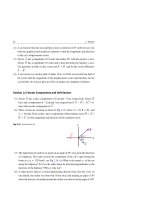
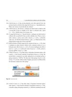
(16) A particle has x = 0 at t = 0 and its velocity as a function of time is shown
in the Fig. 3.21. (a) Sketch the acceleration as a function of time. (b) Find
the average acceleration of the particle in the time interval ti = 0 to tf = 5 s.
(c) Find the acceleration of the particle at t = 4 s.
Fig. 3.21 See Exercise (16)

6

(m/s)

4
2
0
1

2

3

4

5

6

7

t(s)

-2
-4

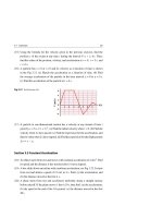
(17) A particle in one-dimensional motion has a velocity at any instant of time t
given by v = 6 + 4 t + 3 t 2 . (a) Find the initial velocity when t = 0. (b) Find the
velocity when 2 s have passed. (c) Find the expression for the acceleration, and
then its value when 2 s have elapsed. (d) Find the expression for the displacement
x = x − x◦ .

Section 3.5 Constant Acceleration
(18) An object starts from rest and moves with constant acceleration of 4 m/s2 . Find
its speed and the distance it has traveled after 5 s have elapsed.
(19) A box slides down an incline with a uniform acceleration, see Fig. 3.22. It starts
from rest and attains a speed of 12 m/s in 4 s. Find: (a) the acceleration, and
(b) the distance moved in the first 4 s.
(20) A plane starts from rest and accelerates uniformly along a straight runway
before takeoff. If the plane moves 1 km in 10 s, then find: (a) the acceleration,
(b) the speed at the end of the 10 s period, (c) the distance moved in the first
20 s.


66

3 Motion in One Dimension

Fig. 3.22 See Exercise (19)

t
°

t

4s

12 m/s

0
0

a

a

(21) A particle moving at 25 m/s in a straight line slows uniformly at a rate of 2 m/s
every second. In an interval of 10 s, find: (a) the acceleration, (b) the final
velocity, (c) the distance moved.

Section 3.6 Free Fall
(22) A stone strikes the ground with a speed of 25 m/s. (a) From what height was it
released? (b) How long was it falling? (c) If the stone is thrown down with a
speed of 10 m/s from the same height, then what will be its speed just before
hitting the ground?
(23) A ball is thrown upward with a speed of 19.6 m/s. (a) How high does it go until
its upward speed decreases to zero? (b) How long does the ball take in this

upward trip? (c) How long does the ball take to return to the initial position?
(d) What will be its velocity then?
(24) A bottle is dropped from a bridge and strikes the water after 5 s. (a) Find the
speed of the bottle when it strikes the water. (b) Find how high the bridge is
located above the water level.
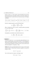
(25) A sandbag dropped from a balloon reaches the ground in 5 s, see Fig. 3.23. Find
the height of the balloon if: (a) it was at rest in the air, (b) it was ascending with
a speed of 10 m/s when the sandbag was dropped, (c) it was descending with a
speed of 10 m/s when the sandbag was dropped.
(26) A ball is thrown vertically downward from the edge of a cliff with an initial
speed of 23 m/s. After a period of 1.4 s has elapsed, find: (a) how fast is it
moving? and (b) how far has it moved?
(27) A ball is thrown vertically upward from the edge of a building with an initial
velocity of 23 m/s. After a period of 1.4 s has elapsed, find: (a) how fast is it
moving? and (b) how far has it moved?
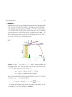
(28) A ball is thrown vertically upward with a speed of 50 m/s from a building 20 m
high, see Fig. 3.24. Find:(a) the time t1 for the ball to reach the highest point,


3.7 Exercises

67

(b) how high it will rise, (c) how long it will take to return to the starting point,
(d) the velocity v2 of the ball at this instant, (e) the velocity v3 with which the
ball strikes the ground, and (f) the total time of flight t3 .
Balloon

Sandbag

Fig. 3.23 See Exercise (25)

Fig. 3.24 See Exercise (28)

O

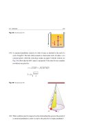
(29) A child drops balls from a bridge at regular intervals of 1s, see Fig. 3.25. At the
moment the fourth ball is released, the first strikes the water. (a) How high is the
bridge? (b) How far above the water are each of the falling balls at this moment:
(c) If the child decided to drop a ball once the previous one has reached the
water surface, how long should he wait between every ball drop?
(30) A rubber ball is released from a height of 2 m above the floor, see the Fig. 3.26.
The ball bounces repeatedly, always rising to 1/2 of the height through which
it falls. Treat the ball as a particle that bounces an infinite number of times and
take g = 10 m/s2 . (a) What is the average speed of the ball during the first fall?
(b) Show that its total distance traveled during an infinite number of bounces
is 6 m? (c) Show that the total elapsed time for an infinite number of bounces


68

3 Motion in One Dimension

√
√
is 2[ 2 + 1]2 / 10 s. (d) Find the average speed from the time of release to
the end of the infinite number of bounces.
[Hint: Use the binomial series (1 − x)−1 = 1 + x + x 2 + x 3 + ..., |x| < 1]
Fig. 3.25 See Exercise (29)

Fourth ball
Third ball

Second ball

First ball

Fig. 3.26 See Exercise (30)

o3 = 0

1m

2m

2=0

o1= 0

o2

1

(31) An acrobat jumps straight up in the air and his center of mass (CM) took 0.2 s
from the moment he just left the ground to the moment he just reached the


3.7 Exercises

69

highest point, see the Fig. 3.27. Neglecting air resistance, (a) what was his
initial vertical velocity just before his legs left the ground, (b) how high did his
CM rise above the ground, and (c) what will be his velocity just before touching
the ground in his way back?
Fig. 3.27 See Exercise (31)

y
Before jump

t= 0 t= 0.2 s

y
CM

(32) Show that the vertical trajectory of a particle thrown upward is symmetric
about its maximum when we neglect air resistance. That is, its height above
the ground at time t before reaching its maximum equals its height above the
ground after the same time interval Δt measured after reaching its maximum.
(33) A student drops a dartboard to the ground from a window, i.e. v◦b = 0. One
second after dropping the board, he throws a dart at the board with initial speed
of 20 m/s in order to score just before the board reaches the ground. See Fig. 3.28
and take g = 10 m/s2 . (a) Find the time of flight T of the dartboard. (b) Find the
height of the window. (c) Find the velocity of both the dart and the dartboard
just before hitting the ground.
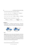
(34) The remote-controlled truck shown in Fig. 3.12 is used to pick up a package
from a shelf in a factory. From rest and at t = 0, the truck accelerate at a1 for
a time interval t1 , then travels with constant speed for a time interval t2 , and
finally decelerate at −a3 for a time interval t3 . Show that the total distance
traveled by the truck is a1 t1 (t2 + t3 ) + 21 (a1 t12 − a3 t32 ).

(35) A diver drops his body from a diving board at a distance H above the water’s
surface into a deep swimming pool. The diver’s motion stops at a distance
h below the surface of the water. By choosing the downward direction to be


70

3 Motion in One Dimension

positive, see Fig. 3.29, prove that the average acceleration of the diver while he
is under the water is a = −(H/h)g.
t=0

t=1s
o=
ob

t=T

20m/s

=0

'b

b

Fig. 3.28 See Exercise (33)

g

mg
o

v =0

H

y
g

mg
w

F
mg h

a
vw′

Fig. 3.29 See Exercise (35)

F
mg
vw= 0


4

Motion in Two Dimensions

This chapter extends the study of the preceding chapter to two dimensions. We divide
the study into two parts: motion of a particle in a plane, and circular motion of a
particle in a plane.

4.1

Position, Displacement, Velocity, and Acceleration Vectors

The Position Vector
→

We describe the position of a particle with the position vector r , which is a vector
that extends from the origin of a certain coordinate system to the particle. Using the
→
unit vector notation of Chap. 2, r can be written in two-dimensional form as:
→

→

→

r = xi + yj

→

→

(4.1)

→

where x i and y j are the vector components of r along the x and y axes respectively,
and the coefficients x and y are the scalar components, i.e., the particle has the
→

rectangular coordinates (x, y). In three dimensions the position vector becomes r =
→
→
→
x i + y j + zk .

The Displacement Vector
Now, consider a particle moving in the xy plane as shown in Fig. 4.1. At point P,
→

→

let its position be r i when the time was ti . At point Q, let its position be r f when
the time was tf (the indices i and f refer to the initial and final values for our study).
Accordingly, during the time interval t = tf − ti , the particle’s displacement is:
→

→

→

r = rf −ri

H. A. Radi and J. O. Rasmussen, Principles of Physics,

Undergraduate Lecture Notes in Physics, DOI: 10.1007/978-3-642-23026-4_4,
© Springer-Verlag Berlin Heidelberg 2013

(4.2)
71


72

4 Motion in Two Dimensions
→

That is, the displacement vector r equals the difference between the final and initial
position vectors. As seen from Fig. 4.1, the magnitude of the displacement vector is
less than the distance traveled along the curved path, which was the particle’s actual
path of motion.
Fig. 4.1 The displacement

y

→
r =→
rf −→
r i of a particle

ti

ticl

P

moving in a plane as it moves

e’s

pat

h
tf

from P to Q during the time
interval

Par

Δr

t = tf − t i

Q

ri
rf

x
O

Average Velocity
One of several quantities associated with the phrase “how fast” a particle moves is
the average velocity, v,

¯ which is defined as follows:
Average velocity
The average velocity, v→, of a particle is defined as the ratio of its displacement,
→
r , to the time interval, t. That is:

v→ =

→

→

→

r
rf −ri
=
t
tf − ti

(4.3)

From this definition, v→, has the dimension of length divided by time, that is m/s
in SI units. It is also a vector quantity that has a magnitude and direction along the
displacement vector

→

r.

Instantaneous Velocity
Consider the motion of a particle between the two points P and Q in the xy
plane, see Fig. 4.2. As the point Q is brought closer and closer to point P (through
points Q 1 , Q 2 , . . .), the time intervals ( t1 , t2 , . . .) get progressively smaller. The
average velocity for each time interval is directed along the displacement vector.
As Q approaches P, the time interval approaches zero, and the direction of the


4.1 Position, Displacement, Velocity, and Acceleration Vectors

73

instantaneous velocity v→, which is the direction of the displacement vector,
approaches the direction of the tangent at P. We define v→as follows:
Instantaneous velocity
The instantaneous velocity, v→, of a particle is defined as the limiting value of
→
the ratio r / t as t approaches zero, i.e.
→

r
t

v→ = lim

t→0

Fig. 4.2 The average velocity
is in the direction of

y

→
r . As

Direction of

Δr

1

→
v approaches the tangent line

ri

to the curve at P

h

at

p
’s

Δr 2

of the instantaneous velocity

le

Q2

tic

→
r and hence the direction

at P

P

ti

r
Pa

Q approaches P, the direction
of

(4.4)

Q1

Δr

r2

Q

r1
rf

x
O
→

In calculus notation, the above limit is called the derivative of r with respect to t,
→
→
and written as d r /dt (simplified as r˙ ). Thus:
v→ =

→

dr
dt

≡

→
rf

→

−ri =

tf

v→ dt

(4.5)

ti

From here on, we use the word velocity to designate instantaneous velocity, and
speed is defined as the magnitude of that velocity.
→
→
→
In unit vector notation, the position vector can be written in the form r = x i + y j ,
and hence we get:
→

→

→

dr
d(x i + y j )
=
v =
dt
dt
→

d x → dy →
=
i +
j

dt
dt

(4.6)


74

4 Motion in Two Dimensions

or
→

→

v→ = vx i + v y j

(4.7)

where the two components of the velocity vector are given by:
dx
,
dt
dy
vy =
dt
vx =

(4.8)

Figure 4.3 shows a velocity vector v→ and its scalar components for a particle moving
in two dimensions.
Fig. 4.3 The velocity →
v

y

of a particle at point P along

t

with its scalar components

rtic
Pa

y

vx and v y

le’s

P
x

h

pat

r

x
O

We should notice that, in a three dimensional study, the velocity vector can be
→
→
→
written in the general form v→ = vx i + v y j + vz k .

Average Acceleration
As the particle moves from P to Q along a certain path in the xy plane as in Fig. 4.4,
its velocity changes from v→i at time ti to v→f at time tf .
We define the average acceleration as:
Average acceleration
→

The average acceleration, a , of a particle is defined as the ratio of the change
in velocity v→ = v→f − v→i to the time interval t = tf − ti . That is:


4.1 Position, Displacement, Velocity, and Acceleration Vectors

y

Part
ic

le’s

ti

75

path

i

tf

P

i

Q
f

ri

f

rf

x
O
Fig. 4.4 The average acceleration →
a for a particle moving from P to Q is in the direction of the change
in velocity

→
v =→

vf −→
v i shown in the right side of the figure

→

a =

v→
v→f − v→i
=
t
tf − ti

(4.9)

→

t is a scalar quantity, the direction of a is in the direction of the change in
velocity v→ = v→f − v→i .
Since

Instantaneous Acceleration
It is useful to define instantaneous acceleration as the limit of the average acceleration
when t approaches zero. When we consider the motion of the particle between the
two points P and Q of the graph shown in Fig. 4.4, we see that as point Q approaches
→

P, the time interval approaches zero, and we define the instantaneous acceleration a
as follows:
Instantaneous acceleration

→
The instantaneous acceleration, a , of a particle is defined as the limiting value
→
of the ratio v→/ t when t approaches zero. Mathematically a can be
expressed as:

→

a = lim

t→0

v→
t

(4.10)


76

4 Motion in Two Dimensions

In calculus notation, the above limit is called the first derivative of v→ with respect
˙ ), or the second derivative of
to t, and written as d v→/dt (simplified sometimes as v→
→
→
→
2
2

r with respect to t, and written as d r /dt (simplified sometimes as r¨ ). Thus:
→

a =

→

d v→
d2r
=
dt
dt 2

≡

v→f − v→i =

tf

→

a dt

(4.11)

ti

From here on, we use the word acceleration to designate instantaneous acceleration.
→
→

In unit vector notation, we use v→ = vx i + v y j , so that:
→

→

d(vx i + v y j )
d v→
=
a =
dt
dt
dvx → dv y →
=
i +
j
dt
dt
→

(4.12)

or
→

→

→

a = ax i + a y j

(4.13)

where the two components of the acceleration vector are given by:
dvx
,
dt
dv y
ay =
dt

ax =

(4.14)

→

Figure 4.5 shows a general view of both the acceleration a and the velocity v→ for
a particle moving in a plane. On the same figure, we display the scalar components
→

of the acceleration vector a .
Fig. 4.5 A general view of

y

rti
Pa

the acceleration vector →
a of a

t

ax

P

ath

particular time t. The figure

p
’s
cle

particle at point P at a

ay

also displays the acceleration

a

scalar components ax and a y ,
as well as the position vector

r

→
r and the velocity vector →

v

O

x


4.1 Position, Displacement, Velocity, and Acceleration Vectors

77

We should notice that in a three dimensional study, the acceleration vector will
→
→
→
→
take the general form a = ax i + a y j + az k .
A particle can accelerate for several reasons. One way is to change with time
the magnitude of the velocity vector (called the speed) such as in one-dimensional
motion. Another way is to change with time the direction of the velocity vector, as
in circular motion. Finally, the acceleration may change due to a change in both the
magnitude and the direction of the velocity vector.
Example 4.1

A particle moves over a path such that the components of its position with respect
to an origin of coordinates are given as a function of time by:
x = −t 2 + 12 t + 5
y = −2 t 2 + 16 t + 10
where t is in seconds and x and y are in meters. (a) Find the particle’s position
→

vector r as a function of time, and find its magnitude and direction at t = 6 s. (b)
Find the particle’s velocity vector v→as a function of time, and find its magnitude
→

and direction at t = 6 s. (c) Find the particle’s acceleration vector a as a function
of time, and find its magnitude and direction at t = 6 s.
Solution: (a) The position vector is given at time t by:
→

→

→

→

→

r = x i + y j = (−t 2 + 12 t + 5) i + (−2 t 2 + 16 t + 10) j

Figure 4.6 shows the variation of x and y as a function of time. At t = 6 s we have:
→

→

→

→

→

r = x i + y j = 41 i + 34 j

→

The magnitude of r is:
x 2 + y2 =

r=

412 + 342 = 53.26 m

→

The angle θ between r and the direction of increasing x is:
θ = tan−1

y
= tan−1
x

34 m
41 m

= tan−1 (0.83) = 39.7◦

Figure 4.7 shows the path of the particle in the xy plane, and also shows its position
→

vector r at t = 6 s.

78

4 Motion in Two Dimensions
Fig. 4.6

50

x

25

meter

0
0

2

4

6

8

10

12

14

t(s)

-25
-50

y

-75
-100

Fig. 4.7

(m)
50
25

r

0
-20

-10 -25 0

10

20

30

(m)
40

-50
-75
-100
-125
-150

(b) The velocity components along the x and y axes are:
d
dx
= (−t 2 + 12 t + 5) = −2 t + 12,
dt
dt

vx =
vy =

d
dy
= (−2 t 2 + 16 t + 10) = −4 t + 16
dt
dt

At t = 6 s the components of v→ are:
vx = 0, v y = −8 m/s
→

That is, v→ = −8 j . The magnitude of v→ at this time is:
v=

vx2 + v 2y =

0 + (−8 m/s)2 = 8 m/s

Hence, the angle θ between v→ and the direction of increasing x is:
θ = tan−1

vy
vx

= tan−1

−8 m/s
0 m/s

= tan−1 (−∞) = 270◦

50


4.1 Position, Displacement, Velocity, and Acceleration Vectors

79

→

where we used the fact that v→ = −8 j is a downward vector and its angle should

be measured in a counterclockwise sense from the direction of increasing x, see
the Fig. 4.7.
(c) The components of the acceleration along the x and y axes are:
ax =

dvx
d
= (−2t + 12) = −2 m/s2 ,
dt
dt

ay =

dv y
d
= (−4t + 16) = −4 m/s2
dt
dt

We see that the acceleration does not vary with time, i.e. it is a constant. We define
→

the magnitude and direction of a as follows:
a=

ax2 + a 2y =
θ = tan−1

(−2 m/s2 )2 + (−4 m/s2 )2 =
ay

ax

−4 m/s2
−2 m/s2

= tan−1

20 (m/s2 )2 = 4.47 m/s2

= 180◦ + tan−1 (2)

= 180◦ + 63.4◦ = 243.4◦
where we used Table 2.1 to calculate θ for a negative ax and a y .

4.2

Projectile Motion

Any object that is thrown into the air is called a projectile. Near the Earth’s surface,
we assume that the downward acceleration due to gravity is constant and the effect
of air resistance is negligible. Based on these two assumptions, we find that: (1) the
horizontal motion and vertical motion are independent of each other and (2) the two
dimensional path of a projectile (also called its trajectory) is always a parabola.
If we choose the axes of the xy plane such that the y axis is vertically upward, then
ax = 0 and a y = −g (as in one-dimensional free fall). Furthermore, let us assume
that at t = 0 the projectile leaves the origin (i.e. x◦ = y◦ = 0) with initial velocity
that makes an angle θ◦ with the positive x direction as in Fig. 4.8.
The projectile’s initial velocity can be written as:

v→◦

→

→

v→◦ = vx◦ i + v y◦ j

(4.15)

The components vx◦ and v y◦ can then be found in terms of the initial speed v◦ and
the launch angle θ◦ as follows:


80

4 Motion in Two Dimensions

t = 12 T

y

y

x°

y

g

y

H

t=T

°

0

0

x°
x°

°

y°

ax
ay

0

x°

x°

x

°

R
y°

Fig. 4.8 The path of a projectile launched from the origin with initial velocity →
v ◦ makes an angle θ◦ with
the x axis. The horizontal velocity component vx◦ remains constant, but the vertical velocity component
v y changes continuously. At the peak of the parabolic trajectory v y = 0 and y is maximum (y = H ). The
horizontal range R is the distance traveled by the projectile when it returns to y = 0

vx◦ = v◦ cos θ◦ ,
v y◦ = v◦ sin θ◦

(4.16)

Now, we decompose the horizontal motion and vertical motion as described below.

Horizontal Motion of a Projectile
Since ax = 0, the horizontal velocity component vx◦ remains constant throughout
the motion, as in Fig. 4.8. Thus, the horizontal velocity vx and the horizontal position
x are described as follows:
vx = vx◦ = constant

⇒

vx = v◦ cos θ◦ = constant

(4.17)

x = vx◦ t

⇒

x = (v◦ cos θ◦ )t

(4.18)

Vertical Motion of a Projectile
Since a y = −g, then the vertical motion is the motion we discussed in Sect. 3.6 for
a particle in free fall. Thus, the vertical velocity v y and the vertical position y can be
described as follows:
v y = v y◦ − gt

⇒

v y = v◦ sin θ◦ − gt

(4.19)


4.2 Projectile Motion

81

y = v y◦ t − 21 gt 2

⇒

y = (v◦ sin θ◦ )t − 21 gt 2

(4.20)

v 2y = v 2y◦ − 2gy

⇒

v 2y = (v◦ sin θ◦ )2 − 2gy

(4.21)

As illustrated in Fig. 4.8, the vertical velocity component v y and the coordinate
y behave like those of an object that is thrown upwards. The initial upward velocity
component steadily decreases reaching zero at the maximum height. The vertical
component then reverses direction, and its magnitude becomes larger with time.

Horizontal Range of a Projectile
The horizontal range R is the distance traveled by the projectile when it returns to
y = 0 after time t = T , as seen in Fig. 4.8. To find an expression for R we use Eq. 4.18
and set x = R at time t = T . We also use Eq. 4.20 and set y = 0. Thus:
R = (v◦ cos θ◦ )T
0 = (v◦ sin θ◦ )T − 21 gT 2
From the last result, we get the following relation for T :
T =

2v◦ sin θ◦
g

(4.22)

Substituting with the expression of T in R = (v◦ cos θ◦ )T and using the identity

sin 2θ◦ = 2 sin θ◦ cos θ◦ , we get:
R=

v◦2 sin 2θ◦
, 0 ≤ θ◦ ≤ π/2
g

(4.23)

The range is maximum when sin 2θ◦ = 1, i.e. when θ◦ = 45◦ , and is the same for
the two angles θ◦ and 90◦ − θ◦ since sin 2θ◦ = sin(180◦ − 2θ◦ ).

Maximum Height of a Projectile
Since the trajectory is symmetric about the peak, then we can find the time t = t1 =
T /2 at the peak from Eq. 4.22. That is:
t1 =

1
2

T =

v◦ sin θ◦
g


82

4 Motion in Two Dimensions

Note that we get the same answer when we set v y = 0 in Eq. 4.19. Substituting with
t1 in Eq. 4.20 we get:
H = (v◦ sin θ◦ )

v◦ sin θ◦
− 21 g
g

v◦ sin θ◦
g

2

Thus:
H=

v◦2 sin2 θ◦
, 0 ≤ θ◦ ≤ π/2
2g

(4.24)

Although θ◦ and 90◦ − θ◦ are two angles that have the same range R, sin θ◦ is not
equal to sin(90◦ − θ◦ ). Therefore, the maximum height H is greater for the bigger
angle. For the same initial speed v◦ , Fig. 4.9 shows these properties by displaying

three trajectories, where two of them are with the same range R when θ◦ = 30◦ and
90◦ − θ◦ = 60◦ , and the third trajectory has a maximum range Rmax when θ◦ = 45◦ .
Fig. 4.9 The trajectories of a

y

projectile fired from the origin

°

with the same initial speed v◦ .
For the two angles θ◦ = 30◦

°

range R, but when θ◦ = 45◦ ,

o

° =45

°

and θ◦ = 60◦ , we get the same

=60

°

o

=30 o

we get the maximum range

Rmax for the projectile motion

0

°

x
R
R max

Equation of the Trajectory
We can find the equation of the projectile’s trajectory by solving Eq. 4.18 for t and
substituting into Eq. 4.20. After performing a few manipulations, we get:
y=

−g
2v◦2 cos2 θ◦

x 2 + (tan θ◦ )x, 0 ≤ θ◦ < π/2

(4.25)

This can be written in the form y = ax 2 + bx, which is the equation of a parabola
that passes through the origin. The angle θ◦ = 90◦ is excluded from Eq. 4.25 since
it represents a projectile that is fired vertically up, i.e. the path of the projectile is a
straight line.


4.2 Projectile Motion

83

Example 4.2

An airplane is flying horizontally with a constant speed v◦ = 400 km/h at a constant elevation h = 2 km above the ground, see Fig. 4.10. (a) If the pilot decided
to release a package of supplies very close to a truck on the ground, then what
is the time of flight of the package? (b) What is the horizontal distance covered
by the package in that time (which is the same horizontal distance covered by the
plane)?
Fig. 4.10

y
o

x

o

h

x

Solution: (a) The initial velocity of the package is the same as the velocity of the
plane. Therefore, the initial velocity of the package v→◦ is horizontal (i.e., θ◦ = 0)
and has a magnitude of 400 km/h. Since we know the vertical distance that the
package falls, then we find its time of flight from Eq. 4.20 as follows:
y = (v◦ sin θ◦ ) t − 21 gt 2
Substituting with y = −2,000 m (we use the negative sign because the package
is bellow the origin) and θ◦ = 0, we get:
−2,000 m = 0 −

1
2

(9.8 m/s2 )t 2

Solving for t and taking the positive root yields:
2,000 m
= 20.2 s
4.9 m/s2
(b) The horizontal distance covered by the package in that time is:
t=

x = (v◦ cos θ◦ ) t
= (400 km/h)(1 h/3600 s)(cos 0◦ )(20.2 s) = 2.244 km
= 2,244 m


84

4 Motion in Two Dimensions

Example 4.3

A basketball player throws a ball at an angle θ◦ = 60◦ above the horizontal, as
shown in the Fig. 4.11. At what speed must he throw the ball to score?
Fig. 4.11

y
vo

o

°

x

2m

3m

4m

Solution: In terms of the unknown speed v◦ , we must first use the horizontal
Eq. 4.18 to find the time needed for the ball to reach the net after moving a
horizontal distance of 4 m. Thus, after omitting the units temporarily since they
are consistent, we get:
x = (v◦ cos θ◦ )t

4 = v◦ (cos 60◦ )t = 0.5v◦ t

⇒

⇒

t=

8
v◦

Since y is up, then a = −g = −9.8 m/s2 during ascending and descending
motions. Also, choosing the origin of the xy plane to be at the player’s hands
makes y◦ = 0. When the ball reaches the net, it gains vertical height y = 1 m.
Then, by using Eq. 4.20 we get:
y = (v◦ sin θ◦ )t − 21 gt 2

⇒

1 = (v◦ sin 60◦ )

8
−
v◦

or,
1 = 6.93 −

313.6
v◦2

Thus, solving for v◦ and taking the positive root gives:
v◦ =

313.6
= 7.27 m/s
6.93 − 1

1
2

× 9.8 ×

8
v◦

2