Hafez a radi, john o rasmussen auth principles of physics for scientists and engineers 19

13.2 Molar Specific Heat Capacity of an Ideal Gas

439

Freely moving piston

Fig. 13.6
Insulation

P
P
P
P

P Vf Tf
QP

P V i Ti
Heat reservoir at T i
Initial

Heat reservoir at Tf
Final

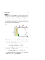
Solution: (a) Treating the helium as an ideal monatomic gas undergoing a
constant-pressure process, we use CP = 20.8 J/mol.K and T = 20 C◦ = 20 K
in Eq. 13.20 to get:
QP = nCP T = n(5R/2) T = (5 mol)(20.8 J/mol.K)(20 K) = 2,080 J
(b) Even though the temperature of the helium increases at a constant pressure
(not at constant volume), we use Eq. 13.23 to calculate the change in internal
energy when CV = 12.5 J/mol.K as follows:

Eint = nCV T = n(3R/2) T = (5 mol)(12.5 J/mol.K)(20 K) = 1,250 J
(c) From the first law of thermodynamics, Eint = QP − W, we calculate the
work done by the gas in this process as follows:
W = QP −

Eint = 2,080 J − 1,250 J = 830 J

Of all the heat energy QP = 2,080 J that is transferred to the helium during the
increase in temperature, only 1,250 J goes to increasing the helium’s internal
energy and hence its temperature. The remaining 830 J is transferred out of the
helium as work done during the expansion.

Internal Energy of a Diatomic Ideal Gas
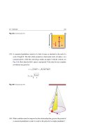
In a diatomic ideal-gas model, a molecule can rotate about two different axes, while
the rotation about the third axis passing through the two atoms gives very little energy
because the moment of inertia about this axis is very small, see Fig. 13.7.
Therefore, a diatomic gas is said to have five energy degrees of freedom: three
translational and two rotational. According to the principle of equipartition of energy,


440

13 Kinetic Theory of Gases

each active degree of freedom of a molecule has on average an energy equal to 21 kB T .
Thus, the average energy for a molecule in a diatomic gas is:
E = 25 kB T

(Diatomic ideal gas)

(13.34)

Very small moment of inertia

Axis

Axis

Axis

Fig. 13.7 A diatomic molecule can rotate about two perpendicular axes with appreciable rotational
energy while the rotation about the third axis gives very little rotational energy (i.e. only two degrees of
freedom)

Hence, the internal energy Eint of a diatomic ideal gas of N (or n kmol) at pressure
P, volume V, and temperature T will be:
Eint =

5
2 NkB T
5
2 nRT

(Diatomic ideal gas)

(13.35)

In general, the internal energy of an ideal gas is a function of T only, and the
exact relationship depends on the type of gas. The vibrational (kinetic and potential) degrees of freedom have only a tiny effect on Eqs. 13.34 and 13.35 unless the
temperature is extremely high. Quantum mechanical study (which is not our aim)

predicts discrete vibrational levels with spacing generally much larger than kB T .
We can use the above results and Eq. 13.25 to find CV and CP as follows:
1 d
1 dEint
=
n dT
n dT
CP = CV + R = 27 R

CV =

5
2 nRT

= 25 R

(Diatomic ideal gas)

(13.36)

Table 13.2 displays the measured molar specific heats of some gases. These results
are in good agreement with the predicted CV and CP . The small deviations from
the predicted values are due to the fact that real gases are not ideal gases. Real
gases experience weak intermolecular interactions, which are not addressed in the
presented ideal gas model.


13.3 Distribution of Molecular Speeds

441

Table 13.2 Some molar specific heats of various gases at 15 ◦ C
Molar specific heat (J/mol C◦ )
Cp

CV

CP − C V

γ = CP /CV

He

20.8

12.5

8.33

1.67

Ar

20.8

12.5

8.33

1.67

Ne

20.8

12.7

8.12

1.64

Kr

20.8

12.3

8.49

1.69

H2

20.8

20.4

8.33

1.41

N2

29.1

20.8

8.33

1.40

O2

29.4

21.1

8.33

1.40

CO

29.3

21.0

8.33

1.40

Cl2

34.7

25.7

8.96

1.35

CO2

37.0

28.5

8.50

1.30

SO2

40.4

31.4

9.00

1.29

H2 O

35.4

27.0

8.37

1.30

Gas
Monatomic gases

Diatomic gases

Triatomic gases

13.3

Distribution of Molecular Speeds

Molecules in a gas at thermal equilibrium are assumed to be in random motion, i.e.
they have a wide range of molecular speeds. In 1859, James Clerk Maxwell derived
an expression that describes the distribution of speeds in a gas containing N molecules
in thermal equilibrium at temperature T. The number of molecules dN with speeds
in the range v and v + dv is defined by the distribution function f (v) (known as
Maxwell-Boltzmann distribution) through the following relation:
dN = f (v) dv = 4π N

m
2π kB T

3/2

1

v 2 e− 2 mv

2 /k

BT

dv

(13.37)

where m is the mass of a gas molecule, kB is Boltzmann’s constant, and T is the
absolute gas temperature. A sketch of the distribution function f (v) is shown in
Fig. 13.8 at a certain temperature T.
The average speed v¯ can be obtained by integrating the product of the speed v
with dN and dividing by the total number N. In addition, one can find vrms and the
most probable speed vp as follows:


442

13 Kinetic Theory of Gases

v¯ =

vrms =

1
N

∞

8 kB T
π m

vf (v) dv =
0

1
N

v2 =

vp =

∞
0

v 2 f (v) dv =

(13.38)
3kB T
m

2kB T
m

(13.39)

(13.40)

From these results, we see that vrms > v¯ > vp as displayed in Fig. 13.8.

f( )

T

p

rms

Fig. 13.8 Distribution of speeds of an ideal gas, f (v). The area under the curve gives the total number
of gas molecules. The speed at the peak vp is less that v¯ and vrms because f (v) is skewed to the right of
the peak

13.4

Non-ideal Gases and Phases of Matter

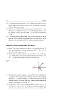
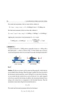
The isothermal PV-diagram presented in Sect. 12.4 and Sect. 13.2 can help us grasp
the overall behavior of a gas described by the gas law PV = nRT . The PV-isotherm for
a constant amount of an ideal gas is displayed for temperatures T4 > T3 > T2 > T1 in
Fig. 13.9a. Notice that the pressure P is inversely proportional to V and that the
isotherms are hyperbolic curves.

Fig. 13.9b displays a PV-diagram for a substance that does not obey the ideal
gas law for temperatures T4 > T3 > Tc > T2 > T1 . The solid curve at T4 represents
the behavior of the non-ideal gas, while the dashed curve represents the behavior
predicted by the ideal gas law at the same temperature. The curves at T3 and Tc deviate
more from the dashed curves predicted by the ideal gas law. At successively lower
temperatures T2 and T1 (both below Tc ), the behavior deviates even more from the
curves of part a, and the isotherms develop flat regions in which the substance can be
compressed without an increase in its pressure. Observation shows that the non-ideal
gas is condensing from vapor (gas) to a liquid state. The colored region represents
isotherms in their liquid-vapor phase equilibrium. A transition from one phase to


13.4 Non-ideal Gases and Phases of Matter

443

another requires phase equilibrium between the two phases. This occurs at only one
definite temperature for a given pressure value.
P

P

Ideal gas

Non-ideal gas
T4 > T3 > Tc > T2 > T1

T4 > T3 > T2 > T1

Isotherms

Isotherms

T4
T3

T4

c
b

T2
T1

V

Liquid

T3

Tc

a
Vapor

Liquid-vapor

(a)

T2

T1

V

(b)

Fig. 13.9 (a) An isothermal P-V diagram of an ideal gas for temperatures T4 > T3 > T2 > T1 . (b) An
isothermal P-V diagram for a non-ideal gas for temperatures T4 > T3 > Tc > T2 > T1 .

Kinetic theory can help us understand this behavior if we note that at higher
pressures, and particularly at lower temperatures, the attractive potential energy due
to attractive forces between molecules cannot be ignored as in the case of an ideal
gas. These attractive forces at lower temperatures tend to pull the molecules and
cause liquefaction.
The curve at Tc in Fig. 13.9b represents the substance at its critical temperature,
and point c on the curve is called the critical point. When we compress the gas at
constant temperature T2 (the volume decreases even more, it begins to liquefy and both the temperature and
pressure remain constant. At point b, the substance is in the liquid state. Note that,
a substance below Tc in the gaseous state is called a vapor, whereas above Tc , it is
called a gas.
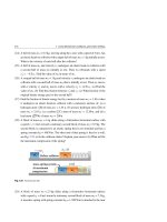
We can represent the condition of phase equilibrium on a PT-diagram such as
that in Fig. 13.10. This diagram is referred to as a phase diagram and displays the
following:
1. The curve labeled L-V represents points where liquid and vapor phases are in
equilibrium (boiling point versus pressure curve)
2. The curve labeled S-L represents points where solid and liquid phases are in
equilibrium (freezing point versus pressure curve)

444

13 Kinetic Theory of Gases

3. The curve labeled S-V represents points where solid and vapor phases are in
equilibrium (sublimation point versus pressure curve)
Fig. 13.10 A P-T diagram of

P

a non-ideal substance showing
regions of temperature and

Critical point

S-L

pressure at which the various
phases exist

Liquid

V

Solid
Solid, liquid, and
vapor coexist

L-

Triple point

V
SVapor

T

All three curves meet at the triple point, the only condition under which all
three phases can coexist. Because the triple point corresponds to a unique value of
temperature and pressure, it is precisely reproducible and is frequently used as a
reference point. In Sect. 11.1, we used the triple-point temperature of water to define
the Kelvin scale. This point occurs at T = 273.16 K and P = 4.58 mm Hg = 6.026 ×
10−3 atm.

13.5

Exercises

Section 13.1 Microscopic Model of an Ideal Gas
(1) In an interval of 1 s, the total number of oxygen molecules that collide perpendicularly with a wall of an area A = 10−3 m2 is N = 5 × 1023 molecules.
Assume that each molecule has a mass m = 5.3 × 10−26 kg and moves with a
perpendicular speed v = 500 m/s. What is the pressure exerted on the wall by
these oxygen molecules?
(2) A 2-mol sample of oxygen gas is at STP [A standard temperature and pressure
implies a temperature of 0 ◦ C (273.15 K) and an atmospheric pressure of 1 atm].
(a) What is the average translational kinetic energy of an oxygen molecule under
these conditions? (b) What is the total translational kinetic energy of the oxygen
molecules?
(3) A gas is at 27 ◦ C. Find the temperature at which the rms (root mean square)
speed of its molecules is doubled.

13.5 Exercises

445

(4) Bellatrix (or Amazon) star is one of the hottest stars that we can see with the
naked eye and its surface temperature is about 3×104 K. (a) Find the rms speed
of helium atoms near the surface of this star. (b) Compare the value of part (a)
with the rms speed at 27 ◦ C.
(5) A vessel of volume V = 4 × 10−2 m3 filled with nitrogen gas contains n = 4 mol
at a pressure P = 2 atm. (a) What is the temperature of this gas? (b) What is
the average translational kinetic energy of a nitrogen molecule under these
conditions?
(6) (a) Use the definition of Avogadro’s number to find the mass of a helium
atom, given that the molar mass of He is 4.00 kg/kmol. (b) How many atoms of
helium are confined in a container of volume V = 10−4 m3 at 27 ◦ C and 1 atm?
(c) What is the rms speed of the helium atoms?
(7) A sample of 2-mol of monatomic argon is at 27 ◦ C. The molar mass of argon
(Ar) is 39.95 kg/kmol. (a) What is the average translational kinetic energy of
an argon atom in this sample? (b) What is the total translational kinetic energy
of all the argon atoms?
(8) At a temperature of 100 ◦ C, a mixture of the monatomic helium and argon gases
is in thermal equilibrium. (a) What is the average kinetic energy for each type
of atom? (b) What is the rms speed for each type of atom? Assume this mixture
displays the properties of an ideal gas, and that the molar mass of helium (He)
is 4.00 kg/kmol, and the molar mass of argon (Ar) is 39.95 kg/kmol.
(9) (a) Find the change in internal energy of n = 4 mol of monatomic neon gas
when its temperature is increased by 10 C◦ . (b) Will your answer change if the
gas is diatomic? Explain your reasoning.

(10) Assume that oxygen at STP is an ideal gas, and that each molecule occupies the
same cubical volume a3 , where a is the length of one side of the cube. (a) Find
the volume of each molecule. (b) Estimate of the average distance between the
oxygen molecules.
√
(11) Find a relation that gives the rms speed vrms = 3RT /M of gas molecules in
terms of the pressure P of the gas and its density ρ.
(12) A sample of nitrogen gas is at 0 ◦ C. (a) What is the rms speed of a nitrogen
molecule at this temperature? (b) Assuming that each molecule has no preferred
direction and does not collide with any other molecule, find the time that one
molecule will cross a cubical container of side a = 1.5 m. (c) Estimate the
number of times that a molecule would move back and forth on the average.


446

13 Kinetic Theory of Gases

Section 13.2 Molar Specific Heat Capacity of an Ideal Gas
(13) A cylinder contains 3 kmol of helium at a temperature of 27 ◦ C. Heat is added
to the gas to increase its temperature to 127 ◦ C, (a) Find the quantity of heat QV
if the gas is heated at a constant volume. (b) As the gas is heated at a constant
pressure, find the amount of added heat QP , the work done by the gas W, and
the increase in internal energy.
(14) A cylinder contains 1 kmol of monatomic ideal gas at initial temperatures of
27 ◦ C, see the Fig. 13.4. In a fixed volume process, QV = 2 × 105 J of heat is
transferred to the gas from a heat reservoir. Find (a) the increase in the internal
energy of the gas, and (b) its final temperature.
(15) A monatomic ideal gas has a specific heat cV = 95.2069 J/kg.C◦ , which is
nearly constant over a wide range of temperatures. What is the molar mass of

the gas? Use the periodic table to find the name of this gas.
(16) A room 4 m × 4.5 m × 2.8 m contains air at 17 ◦ C and 1 atm. Assume that the
air in the room is an ideal diatomic gas with a molar specific heat at constant
volume CV = 20.79 × 103 J/kmol.K. Also assume that there is no air or heat
loss to the outside. If a heater in the room supplies 106 J/h, by how much will
the temperature of the room rise in one hour?
(17) A two mol of an ideal diatomic gas at 20 ◦ C is heated to 70 ◦ C at constant
pressure of 1 atm. (a) What is the change in the internal energy? (b) What is
the work done by the gas? (c) Determine the quantity of heat added to the gas?
(18) A four mol of an ideal diatomic gas is at −30 ◦ C. Assume that all the active
degrees of freedom are three translational, two rotational, and two vibrational.
What is the internal energy of the gas?
(19) Assume that a molecule in an ideal gas has α active degrees of freedom. Show
that for n moles of this gas, the principle of equipartition theory predicts that:
(a) the total internal energy is Eint = 21 αnRT ; (b) the molar specific heat at
constant volume is CV = 21 αR; (c) the molar specific heat at constant pressure
is CP = 21 (α+2)R; (d) the molar specific heat ratio is γ = CP /CV = (α+2)/α.
(20) The diatomic molecule of chlorine (Cl2 ) has a molar mass M = 70 kg/kmol.
The distance between two chlorine atoms is d = 2 × 10−10 m. These two atoms
rotate about their center of mass with an angular speed ω = 2 × 1012 rad/s, see
Fig. 13.11. What is the rotational kinetic energy of such a molecule?
(21) A cylinder contains 2 moles of air (a diatomic ideal gas) of volume
V = 6 × 10−3 m3 at 27 ◦ C. At constant pressure, the air undergoes a volume


13.5 Exercises

447

expansion due to the addition of heat QP = 5 kJ, as shown in Fig. 13.12. (a) Use

Table 13.2 to find the values of CP and CV for air, if air contains 78.08% N2 ,
20.95% O2 , 0.93% Ar, and 0.03% CO2 . (b) Find the change in temperature.
(c) What is the change
volume of the air.

Eint of the internal energy of the air? (d) Find the final

Fig. 13.11 See Exercise (20)

Axis

ω
Cl

Cl

Freely moving piston

d

Insulation

P
P

P
P
P V i Ti
Heat reservoir at T i
Initial

P Vf Tf
QP
Heat reservoir at Tf
Final

Fig. 13.12 See Exercise (21)

Section 13.3 Distribution of Molecular Speeds
(22) For the Maxwell-Boltzmann speed distribution given by Eq. 13.37 and displayed in Fig. 13.8, the most probable speed vp of a gas molecule corresponds
to a point on the curve at which the slope is zero, i.e. when the condition
df (v)/dv|v = vp = 0 is fulfilled. Use this condition to show that vp is given by
Eq. 13.40.
(23) A container is filled with oxygen gas at T = 300 K. (a) Find the rms speed
vrms of the oxygen molecule. (a) What is the average speed v¯ of the oxygen
molecule? (c) Find the value of the most probable speed vp ?


448

13 Kinetic Theory of Gases

(24) The rms speed vrms of a gas at temperature T1 is equal to the most probable
speed vp at temperature T2 . Evaluate the ratio T2 /T1 .
(25) A container is composed of N = 106 oxygen molecules at T = 300 K. Assume
that the gas obeys the Maxwell’s speed distribution and the oxygen molecule has
a mass m = 5.31 × 10−26 kg. Calculate the number of molecules with speeds
between: (a) 300 m/s and 301 m/s; (b) 1,000 m/s and 1,001 m/s.

Part IV

Sound and Light Waves


14

Oscillations and Wave Motion

Any object that repeats its motion at regular time intervals is said to perform a
periodic or harmonic motion. If the motion is a sinusoidal function of time, we call
it simple harmonic motion.

14.1

Simple Harmonic Motion

Assume the motion of a particle moving back and forth about the origin o of the
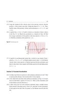
x-axis between the limits x = +A and x = −A, as shown in Fig. 14.1.

-A

o

A

x

One complete cycle

t=0
t = T/4
t = T/2
t = 3T/4
t=T
Fig. 14.1 Multiple snapshots of a particle oscillating about the origin of the x-axis between the two limits
x = + A and x = − A. If the time t = 0 is chosen to be when the particle is at x = + A, then the particle
returns to x = + A when t = T , where T is the period of the motion

In this figure, we chose t = 0 at the point where the particle is at x = +A
and t = T when the particle returns to the same point x = +A after one complete
H. A. Radi and J. O. Rasmussen, Principles of Physics,
Undergraduate Lecture Notes in Physics, DOI: 10.1007/978-3-642-23026-4_14,
© Springer-Verlag Berlin Heidelberg 2013

451


452

14 Oscillations and Wave Motion

cycle. In this case, T represents the period of the motion. The frequency f of
the simple harmonic motion is equal to the number of oscillations per unit time.
Therefore, the frequency is related to the period T by the following relation:
f =

1
T

(Harmonic motion)

(14.1)

and has the SI unit s−1 , cycle/s, or hertz (Hz). Additionally, we define the angular
frequency of the motion by the relation:
ω=

2π
T

(Harmonic motion)

(14.2)

Accordingly, this relation can be written in terms of the frequency f as follows:
ω = 2π f

(Harmonic motion)

(14.3)

where the SI unit of ω is rad/s. For such a motion, the displacement x of the particle
from o is given generally as a function of time as:
x(t) = A cos(ω t + φ)

(14.4)

where A is the amplitude of the motion and φ is the phase angle or phase constant
(φ is zero in Fig. 14.1). The cosine function in Eq. 14.4 varies between the limits ±1,

so the displacement x(t) varies between the limits ±A, as shown in Fig. 14.2.

x
φ =0

+A

φ = -π /4

A
t

o
A
-A

Τ

Fig. 14.2 A sketch of the relation x(t) = A cos(ω t + φ) for φ = 0 and φ = −π/4

14.1.1 Velocity and Acceleration of SHM
We can find an expression for the velocity v of a particle moving with a harmonic
motion by differentiating Eq. 14.4 as follows:


14.1 Simple Harmonic Motion

453

v(t) =

d[A cos(ω t + φ)]
dx
=
dt
dt

Thus:
v(t) = −ω A sin(ω t + φ) = −vmax sin(ω t + φ) ,

vmax = ω A

(14.5)

By differentiating this expression, we generate the following expression for the acceleration of the oscillating particle:
a(t) =

d[−ω A sin(ω t + φ)]
dv
=
dt
dt

Thus:
a(t) = −ω2 A cos(ω t + φ) = −amax cos(ω t + φ) ,

amax = ω2 A

(14.6)

Figure 14.3 shows a plot of Eqs. 14.4–14.6 for φ = 0.

Τ

+A

Position x

A

o

x = A cos(ω t )
t

A
-A

Velocity

+ω A

= -ω A sin(ω t )
o

t

Acceleration a

-ω A

a = -ω 2 A cos(ω t )

+ ω 2A

o

t

- ω 2A

Fig. 14.3 The upper part of the figure shows the variation of the displacement x(t) with time t of
a particle oscillating with a SHM when the phase angle φ is equal to zero. The middle and lower
parts display the variation of v(t) and a(t) with time. In all parts of the figure, the period T marks one
complete oscillation


454

14 Oscillations and Wave Motion

Example 14.1

A particle oscillates with a simple harmonic motion along the x axis. Its displacement from the origin varies with time according to the equation:
x = (2 m) cos(0.5π t + π/3)
where t is in seconds and the argument of the cosine is in radians. (a) Find the
amplitude, frequency, and period of the motion. (b) Find the velocity and acceleration of the particle at any time. (c) Find both the maximum speed and acceleration
of the particle. (d) Find the displacement of the particle between t = 0 and t = 2 s.
Solution: (a) By comparing the given equation to the general form x(t) =
A cos (ω t + φ), we find that: the amplitude A = 2 m, the angular frequency

ω = 0.5π rad/s, and the phase constant φ = π/3 rad.
Therefore, the frequency will be:
f = ω/2π = (0.5π rad/s)/(2π rad) = 0.25 s−1 = 0.25 Hz
Hence the period will be given by:
T = 1/f = 1/0.25 s−1 = 4 s
(b) We differentiate x to find v, and then v to find a, as follows:
d[(2 m) cos(0.5π t + π/3)]
dx
=
dt
dt
= (2 m)[−sin(0.5π t + π/3)] × (0.5π rad/s)

v=

= −(π m/s) sin(0.5π t + π/3)
d[(−π m/s) sin(0.5π t + π/3)]
dv
=
dt
dt
= (−π m/s)[cos(0.5π t + π/3)] × (0.5π rad/s)

a=

= −(0.5π 2 m/s2 ) cos (0.5π t + π/3)
Remember, the rad is a dimensionless quantity and can be removed from or
inserted into any calculation without altering the dimension of the result.
(c) Since the maximum values of the sine and cosine are unity, then v of part
(b) varies between ± π m/s, and a of part (b) varies between ±0.5π 2 m/s2 . Thus,

the maximum speed and maximum acceleration are as follows:


14.1 Simple Harmonic Motion

455

vmax = π m/s
amax = 0.5π 2 m/s2
We can also use Eqs. 14.5 and 14.6 to find vmax and amax as follows:
vmax = ω A = (0.5π rad/s)(2 m) = π m/s
amax = ω2 A = (0.5π rad/s)2 (2 m) = 0.5π 2 m/s2
(d) The position of the particle at t = 0 is denoted by xi and is given by:
xi = (2 m) cos(0 + π/3) = (2 m)(0.5) = 1 m
The position of the particle at t = 2 s is denoted by xf and is given by:
xf = (2 m) cos(π + π/3) = (2 m)(−0.5) = −1 m
Therefore, the displacement between t = 0 and t = 2 s is:
x = xf − xi = −1 m − 1 m = −2 m
Figure 14.4a shows the plot of x versus t for the given function, while Fig. 14.4b
depicts snapshots of the oscillating particle about the origin of the x-axis between
the two limits x = +2 m and x = −2 m.
-2 m

2

xi

1

x(m)

xf

-1 m

o

+1 m

t=0

xi

t = 2s

+2 m

x
t=0

0

-2

t=2s

xf

-1

t (s)

0

1

2

3

t=4s

4

(a)

(b)

Fig. 14.4

14.1.2 The Force Law for SHM
We can combine Eqs. 14.4 and 14.6 to yield:
a(t) = −ω2 x(t)

(14.7)


456

14 Oscillations and Wave Motion

This equation is the hallmark of simple harmonic motion. It states that the acceleration

is proportional to the displacement but opposite in sign, and they are related by the
square of the angular frequency, ω2 .
Once we know the acceleration as a function of time, we can use Newton’s second
law to find what force must act on the particle to produce this acceleration. Now, we
combine Newton’s second law with Eq. 14.7 as follows:
F = m a = −(m ω2 )x or

d2x
+ ω2 x = 0
dt 2

(14.8)

This form (a force proportional to the displacement but opposite in sign) is familiar
to us. It is Hooke’s law for a spring, which was introduced in Sect. 6.3. That is:
F = −kH x

(Hooke’s law)

(14.9)

By comparison, the equivalent spring constant in SHM is:
kH = m ω2

(14.10)

We can take Eq. 14.9 as an alternative definition of SHM.
Simple Harmonic Motion
SHM is the motion executed by a particle of mass m subject to a force proportional to its displacement but opposite in sign.

The block-spring system of Fig. 14.5 forms a linear simple harmonic oscillator.
The angular frequency ω of the simple harmonic motion is related to the spring
constant kH and the mass of the block by Eq. 14.10, which gives:
ω=

kH
m

(14.11)

Therefore, using Eqs. 14.5, 14.6, and 14.11, we can find the maximum values for
the velocity and acceleration of the oscillations as follows:
vmax = ω A =

amax = ω2 A =

kH
A
m

(14.12)

kH
A
m

(14.13)


14.1 Simple Harmonic Motion

Fig. 14.5 The variation of the

457

Equilibrium position

(a)

force of a spring on a block.
(a) When x = 0, the force is

F=0
x=0

x

zero (equilibrium position).
(b) When x is negative, the

x=0

force is positive (compressed
spring). (c) When x is positive,

(b)

F

the force is negative (stretched
spring)

Positive F
Negative x

x
x
(c)

x=0

F

Negative F
Positive x

x
x=0

x

By combining Eqs. 14.2 and 14.11, we can find the period T of the oscillations as
follows:
T=

2π
= 2π
ω

m
kH

(14.14)

That is, the period T and hence the frequency f = 1/T depend only on the mass of
the particle m and the spring constant kH , and not on the parameters of the motion,
such as A or φ.
Example 14.2

A block of mass m = 400 g is attached to a light spring of force constant
kH = 10 N/m, see Fig. 14.6a. The block is pushed against the spring from x = 0 to
xi = −10 cm, see Fig. 14.6b, and then released to oscillate on a horizontal frictionless surface. (a) Find the angular frequency and the period of the block-spring
system. (b) Find the maximum speed and maximum acceleration of the block. (c)
Find the position, speed, and acceleration of the block at any time. (d) Repeat the
above parts when the block is projected with initial velocity vi = −0.5 m/s from
another initial position xi = +10 cm.


458

14 Oscillations and Wave Motion

Fig. 14.6

(a)

Equilibrium position

x

x=0

(b)

x

xi

x=0

Solution: (a) Using Eqs. 14.11 and 14.14 we find the angular frequency and the
period of motion as follows:
ω=
T=

kH
=
m

10 N/m
= 5 rad/s
400 × 10−3 kg

2 × 3.1416 rad
2π
=
= 1.26 s
ω
5 rad/s

(b) Since A = |xi | = 10 cm, then Eqs. 14.12 and 14.13 will give:
vmax = ω A = (5 rad/s)(0.1 m) = 0.5 m/s

amax = ω2 A = (5 rad/s)2 (0.1 m) = 2.5 m/s2
(c) We can find the phase constant φ when we apply the initial condition
x(0) = −A at t = 0 to the form x(t) = A cos(ω t + φ). Thus:
x(t) = A cos(ω t + φ) ⇒ x(0) = A cos(φ) ⇒ − A = A cos(φ) ⇒ φ = π
Therefore, x(t) = A cos(ω t + π ). Using this expression and the results of parts
(a) and (b), we get:
x(t) = A cos(ω t + π ) = (0.1 m) cos(5 t + π )
v(t) = −ω A sin(ω t + π ) = −(0.5 m/s) sin(5 t + π )
a(t) = −ω2 A cos(ω t + π ) = −(2.5 m/s2 ) cos(5 t + π )


14.1 Simple Harmonic Motion

459

(d) In this case, we start with the general form x(t) = A cos(ω t + φ),
where A and φ are not known, but ω does not change because it is independent of
how the oscillation is set into motion. Thus:
(1) x(0) = A cos(0 + φ) = xi
(2) v(0) = −ω A sin(0 + φ) = vi
Dividing Eq. (2) by Eq. (1) gives a phase-constant relation:
vi
−ω A sin(φ)
=
A cos(φ)
xi
Thus:

⇒

tan(φ) = −

vi
−0.5 m/s
=1
=−
ω xi
(5 rad/s)(0.1 m)

φ = tan−1 (1) = 0.785 rad = 0.25 π rad

Now, Eq. (1) allows us to find the new amplitude A as follows:
A=

(0.1 m)
xi
=
= 0.14 m = 14 cm
cos(φ)
cos(0.25π )

The new maximum speed and acceleration will be:
vmax = ω A = (5 rad/s)(0.14 m) = 0.7 m/s
amax = ω2 A = (5 rad/s)2 (0.14 m) = 3.5 m/s2
Finally, the new expressions for x, v, and a are as follows:
x(t) = A cos(ω t + φ) = (0.14 m) cos(5 t + 0.25π )
v(t) = −ω A sin(ω t + φ) = −(0.7 m/s) sin(5 t + 0.25π )
a(t) = −ω2 A cos(ω t + φ) = −(3.5 m/s2 ) cos(5 t + 0.25π )

14.1.3 Energy of the Simple Harmonic Oscillator

Consider the block-spring system shown in Fig. 14.6 when the spring is massless
and the horizontal surface is frictionless (known as the linear oscillator). In such a
situation, the kinetic energy of the system is associated entirely with the block. Its
value depends only on the velocity v given by Eq. 14.5. Thus:
K = 21 mv 2 = 21 mω2 A2 sin2 (ω t + φ)

(14.15)


460

14 Oscillations and Wave Motion

When using Eq. 14.11 to substitute kH /m for ω2 , we find:
K = 21 mv 2 = 21 kH A2 sin2 (ω t + φ)

(14.16)

On the other hand, the potential energy of the linear oscillator of Fig. 14.6 is
associated entirely with the spring. Its value depends only on the position x given by
Eq. 14.4. Thus:
U = 21 kH x 2 = 21 kH A2 cos2 (ω t + φ)

(14.17)

The mechanical energy E of the simple harmonic oscillator is thus:
E = K + U = 21 kH A2 sin2 (ω t + φ) + 21 kH A2 cos2 (ω t + φ)
= 21 kH A2 [sin2 (ω t + φ) + cos2 (ω t + φ)]

(14.18)

When we use the identity sin2 θ + cos2 θ = 1, we find:
E = K + U = 21 kH A2

(14.19)

That is, the mechanical energy (or the total energy) of a simple harmonic oscillator
is constant, independent of time, and is proportional to the square of the amplitude.
Because v = 0 at x = ± A, i.e. K = 0, the mechanical energy equals the maximum
potential energy, i.e. E = Umax = 21 kH A2 . At the equilibrium position x = 0 we have
U = 0, and the mechanical energy equals the maximum kinetic energy, i.e. E =
2 = 1 k A2 .
Kmax = 21 mvmax
2 H
Since the potential energy U is expressed as a function of the position x through
the relation U = 21 kH x 2 , then Eq. 14.19 allows us of to express the kinetic energy as
a function of x as follows:
K = E − U = 21 kH A2 − 21 kH x 2 = 21 kH (A2 − x 2 )

(14.20)

Figure 14.7a displays both the kinetic energy K and potential energy U as a
function of time t, while Fig. 14.7b displays the variation of K and U as a function
of position x.
Finally, by using Eq. 14.20 we can find the velocity of the block at any arbitrary
position x as follows:
K = 21 mv 2 = 21 kH (A2 − x 2 )

v=±

kH 2
(A − x 2 )
m

(14.21)


14.1 Simple Harmonic Motion

461

f=0

K, U

K, U
K(t ) + U(t )

1 k A2
2 H

K(x) + U(x)
1 k A2
2 H

U(t )

U(x )

K(t )

K(x)

x

t
0

T/ 2

T

-A

(a)

0

A

(b)

Fig. 14.7 (a) The kinetic energy K(t) and the potential energy U(t) as a function of time when φ = 0
for a simple harmonic oscillator. Note that K(t) and U(t) peak twice during every period. (b) The kinetic
energy K(x) and the potential energy U(x) as a function of x. For x = 0 the energy is entirely kinetic, and
for x = ±A it is entirely potential

When using Eq. 14.11 to substitute kH /m for ω2 , we find:
v = ±ω

(A2 − x 2 )

(14.22)

This relation verifies the fact that the speed is a maximum when x = 0 and is zero at
both of the turning points x = ± A.
Example 14.3

A block of mass m = 320 g is fastened to a light spring whose force constant
kH is 72 N/m, see Fig. 14.8a. The block is pulled a distance xi = 50 cm from its
equilibrium position at x = 0 on a horizontal frictionless surface, see Fig. 14.8b,
and released at t = 0. (a) What is the mechanical energy of the oscillating block?
(b) What is the maximum speed of the oscillating block? (c) Find the velocity,
kinetic energy, and potential energy of the block when its position is 30 cm?
Equilibrium position

x

x=0

(a)
Fig. 14.8

x

x=0

(b)

xi

462

14 Oscillations and Wave Motion

Solution: (a) Since A = xi = 50 cm = 0.5 m, then Eq. 14.19 gives:
E = 21 kH A2 = 21 (72 N/m)(0.5 m)2 = 9 J
2 ; therefore:
(b) At x = 0, we know that U = 0 and E = 21 mvmax
2
1
2 mvmax

vmax =

=E=9J

2E
=
m

2(9 J)
= 7.5 m/s
0.32 kg

(c) We use Eq. 14.21 to find the velocity at x = 30 cm as follows:
v=±

kH 2

72 N/m
(A − x 2 ) = ±
[(0.5 m)2 − (0.3 m)2 ] = ±6 m/s
m
0.32 kg

Now, we can find K and U when x = 30 cm = 0.3 m as follows:
K = 21 mv 2 = 21 (0.32 kg)(±6 m/s)2 = 5.76 J
U = 21 kH x 2 = 21 (72 N/m)(0.3 m)2 = 3.24 J

14.2

∗

Damped Simple Harmonic Motion

When non-conservative forces, such as friction, oppose the motion of an oscillator,
its mechanical energy diminishes with time, and the motion is said to be damped.
One such system is a block of mass m attached to a spring and immersed in a viscous
liquid, see Fig. 14.9a. Let us assume that the liquid exerts a damping force Fd that is
proportional to the velocity vx of the oscillator. If vx is small, then:
Fd = −bvx

(14.23)

where b is a damping constant. The total force acting on the block is:
Fx = −kH x − bvx
If we set vx = dx/dt and substitute with Fx in Newton’s second law,
m d 2 x/dt 2 , we find the following differential equation:
m

d2x
dx
+ b + kH x = 0
dt 2
dt

(14.24)
Fx =

(14.25)


14.2

Damped Simple Harmonic Motion

(a)

463

(b) x
A

φ=0

Ae − (b/2m)t
t

0

m
x

Fig. 14.9 (a) A damped oscillator consisting of a block immersed in a viscous liquid. (b) Graph of x
versus t for a damped oscillator

This equation has a solution displayed in Fig. 14.9b, and is given by:
x(t) = Ae−bt/2m cos(ωd t + φ)

(14.26)

where the angular frequency of the damped oscillator ωd is given by:
ωd =

14.3

kH
b2
−
m
4m2

√
b 2 kH m

ωd −−−−−−→
or b→0

kH
=ω

m

(14.27)

Sinusoidal Waves

Waves are of three types: mechanical, electromagnetic, and matter waves. This
chapter deals only with mechanical waves. We encounter mechanical waves almost
constantly every day in our lives. For such waves, information and energy move
from one point to another, but matter does not. Common examples of such waves
are sound, water, and seismic waves. These waves require the following:
(1) Some source of disturbance (or vibration),
(2) A medium that can be disturbed,
(3) Some physical mechanism responsible for allowing adjacent portions of the
medium to influence each other.

14.3.1 Transverse and Longitudinal Waves
Figure 14.10 displays a single pulse wave sent from one end of a long stretched
string toward the other fixed end. As the wave passes the point P on the string, the y


464

14 Oscillations and Wave Motion

coordinate of this point will increase, reach a maximum, and then decrease to zero.
In the case of an ideal string (that is when no frictional forces within the string cause
the pulse to die out as it travels), the wave pulse in the string moves along the string
with some constant velocity v.

y
At time t

P

x

Fig. 14.10 Sending a single pulse through a long stretched string

Figure 14.11 displays a continuous sinusoidal wave sent from one end of a long
stretched string toward the other fixed end. The wave has a sinusoidal shape at any
time. That is, the wave has the shape of a sine curve (or a cosine curve) at any
location x and time t. As the sinusoidal wave travels along the string with some
constant velocity v→, the y coordinate of point P on the string will oscillate up and
down continuously.

y
At time t

P

x

Fig. 14.11 Sending a continuous sinusoidal wave through a long stretched string. Any string element
(represented by point P) oscillates perpendicular to the direction of the wave’s velocity

From Figs. 1.10 and 1.11 we find that the displacement of every oscillating element
on the string is perpendicular to the direction of the wave’s velocity. This motion is
called a transverse motion, and the generated wave is called a transverse wave.
Figure 14.12 shows how we can produce a sound wave by using a movable piston

fitted in a long open pipe filled with air. A sound wave can be generated by pushing