Hafez a radi, john o rasmussen auth principles of physics for scientists and engineers 26

19.4 Exercises

653

(13) Silver has 47 electrons per atom and a molar mass of 107.87 kg/kmol. An
electrically neutral pin of silver has a mass of 10 g. (a) Calculate the number of
electrons in the silver pin (Avogadro’s number is 6.022 × 1026 atoms/kmol).
(b) Electrons are added to the pin until the net charge is −1 mC. How many
electrons are added for every billion (109 ) electrons in the neutral atoms?
(14) Two protons in an atomic nucleus are separated by 2 × 10−15 m (a typical internuclear dimension). (a) Find the magnitude of the electrostatic repulsive force
between the protons. (b) How does the magnitude of the electrostatic force
compare to the magnitude of the gravitational force between the two protons?
(15) Two particles have an identical charge q and an identical mass m. What must
the charge-mass ratio, q/m, of the two particles be if the magnitude of their
electrostatic force equals the magnitude of the gravitational force.
(16) Two equally charged pith balls are at a distance r = 3 cm apart, as shown in
Fig. 19.17. Find the magnitude of the charge on each ball if they repel each
other with a force of magnitude 2 × 10−5 N. Does the answer give you any hint
about the exact sign of each charge? Explain.
Fig. 19.17 See Exercise (16)

q

q

r
(17) Two point charges q1 and q2 are 3 m apart, and their combined charge is 40 μC.
(a) If one repels the other with a force of 0.175 N, what are the two charges?
(b) If one attracts the other with a force of 0.225 N, what are the two charges?
(18) Two point charges q1 = +4 μC and q2 = +6 μC are 10 cm apart. A point charge
q3 = +2 μC is placed midway between q1 and q2 . Find the magnitude and

direction of the resultant force on q3 .
(19) Three 4 μC point charges are placed along a straight line as shown in Fig. 19.18.
Calculate the net force on each charge.
(20) Three point charges q1 = q2 = q3 = −4 μC are located at the corners of an
equilateral triangle as shown in Fig. 19.19. (a) Calculate the magnitude of


654

19 Electric Force

the net force on any one of the three charges. (b) If the charges are positive, i.e. q1 = q2 = q3 = +4 μC, would this change the magnitude calculated in
part a?
Fig. 19.18 See Exercise (19)

q 1 =+ 4 C

q 2 =+ 4 C

q 3 =+ 4 C

+

+

+

3m

3m

Fig. 19.19 See Exercise (20)

q1

–
1m

1m

–
q

3

–

1m

q

2

(21) Three point charges q1 = +2 μC, q2 = −3 μC, and q3 = + 4 μC are located at
the corners of a right angle triangle as shown in Fig. 19.20. Find the magnitude
and direction of the resultant force on q3 .
Fig. 19.20 See Exercise (21)

q1 +

y
x

5cm
q2 –

30°

+ q3

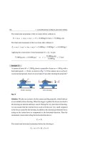
(22) Three equal point charges of magnitude q lie on a semicircle of radius R as
√
shown in Fig. 19.21. Show that the net force on q2 has a magnitude kq2 / 2R2
and points downward away from the center C of the semicircle.
(23) Four equal point charges, q1 = q2 = q3 = q4 = +3 μC, are placed at the four
corners of a square that has a side a = 0.4 m, see Fig. 19.22. (a) Find the force


19.4 Exercises

655

on q1 . (b) Find the force exerted on a test charge of 1 C placed at the center P
of the square.
Fig. 19.21 See Exercise (22)

q1

q3

R

C

R

q2

Fig. 19.22 See Exercise (23)

q1

+

+ q4

y

x

P

q2

+ a = 0.4m + q 3

(24) Four equal point charges q1 = q2 = q3 = q4 = −1 μC, are located as shown in
Fig. 19.23. (a) Calculate the net force exerted on the charge q4 , which is located
midway between q1 and q3 . (b) Calculate the magnitude and direction of the
net force on the charge q2 .

Fig. 19.23 See Exercise (24)

q1

–

y
x

–

1m
q2

–

1m

q4

–

q3

(25) A negative point charge of magnitude q is located on the x-axis at point x = −a,
and a positive point charge of the same magnitude is located at x = +a, see Fig.
19.24. A third positive point charge q◦ is located on the y-axis with a coordinate


656

19 Electric Force

(0, y). (a) What is the magnitude and direction of the force exerted on q◦ when
it is at the origin (0,0)? (b) What is the force on q◦ when its coordinate is (0, y)?
(c) Sketch a graph of the force on q◦ as a function of y, for values of y between
−4a and +4a.
Fig. 19.24 See Exercise (25)

y

+ + qo
y

r−
-q

–

θ

r+
θ

+q

+

0

(-a,0 )

x

(a,0 )

(26) In the Bohr model of the hydrogen atom, an electron of mass m = 9.11 ×
10−31 kg revolves about a stationary proton in a circular orbit of radius
r = 5.29 × 10−11 m, see Fig. 19.25. (a) What is the magnitude of the electrical
force on the electron? (b) What is the magnitude of the centripetal acceleration
of the electron? (c) What is the orbital speed of the electron?
Fig. 19.25 See Exercise (26)

Electron

r

Fe
Fe

Proton

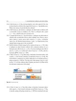
(27) In the cesium chloride crystal (CsCl), eight Cs+ ions are located at the corners
of a cube of side a = 0.4 nm and a Cl− ion is at the center, see Fig. 19.26. What
is the magnitude of the electrostatic force exerted on the Cl− ion by: (a) the
eight Cs+ ions?, (b) only seven Cs+ ions?
(28) Two positive point charges q1 and q2 are set apart by a fixed distance d and
have a sum Q = q1 + q2 . For what values of the two charges is the Coulomb
force maximum between them?

19.4 Exercises

657

Fig. 19.26 See Exercise (27)

a
Cs
Cl

(29) Two equal positive charges q are held stationary on the x-axis, one at x = − a
and the other at x = +a. A third charge +q of mass m is in equilibrium at x = 0
and constrained to move only along the x-axis. The charge +q is then displaced
from the origin to a small distance x a and released, see Fig. 19.27. (a) Show
that +q will execute a simple harmonic motion and find an expression for its
period T. (b) If all three charges are singly-ionized atoms (q = q = +e) each of
mass m = 3.8 × 10−25 kg and a = 3 × 10−10 m, find the oscillation period T.

Fig. 19.27 See Exercise (29)

+ q′

+q
0

+q

x

a

a

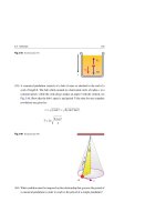
(30) Two identical small spheres of mass m and charge q hang from non-conducting
strings, each of length L. At equilibrium, each string makes an angle θ with
the vertical, see Fig. 19.28. (a) When θ is so small that tan θ sin θ , show that
the separation distance r between the spheres is r = (Lq2 /2π ◦ mg)1/3 . (b) If
L = 10 cm, m = 2 g, and r = 1.7 cm, what is the value of q?

Fig. 19.28 See Exercise (30)

θ

L

q

L

θ
x

x
r

q


658

19 Electric Force

(31) For the charge distribution shown in Fig. 19.29, the long non-conducting massless rod of length L (which is pivoted at its center) is balanced horizontally
when a weight W is placed at a distance x from the center. (a) Find the distance
x and the force exerted by the rod on the pivot. (b) What is the value of h when
the rod exerts no force on the pivot?
Fig. 19.29 See Exercise (31)

L
x
+q

+2q

h

W

Pivot

h

+Q

+Q

(32) Two small charged spheres hang from threads of equal length L. The first sphere
has a positive charge q, mass m, and makes a small angle θ1 with the vertical,
while the second sphere has a positive charge 2 q, mass 3m, and makes a smaller

angle θ2 with the vertical, see Fig. 19.30. For small angles, take tan θ θ and
assume that the spheres only have horizontal displacements and hence the
electric force of repulsion is always horizontal. (a) Find the ratio θ1 /θ2 . (b)
Find the distance r between the spheres.
Fig. 19.30 See Exercise (32)

L

T1

L

θ1

θ2

m

T2
3m

q

2q
r


20

Electric Fields

In this chapter, we introduce the concept of an electric field associated with a variety
of charge distributions. We follow that by introducing the concept of an electric field
in terms of Faraday’s electric field lines. In addition, we study the motion of a charged
particle in a uniform electric field.

20.1

The Electric Field

Based on the electric force between charged objects, the concept of an electric field
was developed by Michael Faraday in the 19th century, and has proven to have
valuable uses as we shall see.
In this approach, an electric field is said to exist in the region of space around
→
any charged object. To visualize this assume an electrical force of repulsion F
between two positive charges q (called source charge) and q◦ (called test charge),
see Fig. 20.1a.
Now, let the charge q◦ be removed from point P where it was formally located as
→

shown in Fig. 20.1b. The charge q is said to set up an electric field E at P, and if q◦
→
is now placed at P, then a force F is exerted on q◦ by the field rather than by q, see
Fig. 20.1c.
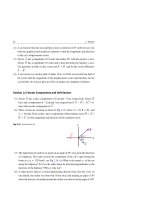
Since force is a vector quantity, the electric field is a vector whose properties are
determined from both the magnitude and the direction of an electric force. We define
→
the electric field vector E as follows:

H. A. Radi and J. O. Rasmussen, Principles of Physics,
Undergraduate Lecture Notes in Physics, DOI: 10.1007/978-3-642-23026-4_20,
© Springer-Verlag Berlin Heidelberg 2013

659


660

20 Electric Fields

Spotlight

→

The electric field vector E at a point in space is defined as the electric
→
force F acting on a positive test charge q◦ located at that point divided by
the magnitude of the test charge:

→

→

E =

F
q◦

Fig. 20.1 (a) A charge q

(20.1)

q

→

+

exerts a force F on a test

+++
+

(a)

charge q◦ at point P. (b) The
→

electric field E established at

qo

+

F

P

P due to the presence of q. (c)

→

→

The force F = q◦ E exerted

q

→

by E on the test charge q◦

+
+++
+

(b)

q

+
+++
+

(c)

P

E

qo

+
P

F = qo E

This equation can be rearranged as follows (see Fig. 20.1c):
→

→

F = q◦ E

(20.2)

→

The SI unit of the electric field E is newton per coulomb (N/C).
→
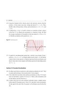
The direction of E is the direction of the force on a positive test charge placed in
the field, see Fig. 20.2.

20.2

The Electric Field of a Point Charge

To find the magnitude and direction of an electric field, we consider a positive point
charge q as a source charge. A positive test charge q◦ is then placed at point P,

20.2 The Electric Field of a Point Charge

661

a distance r away from q, see Fig. 20.3. From Coulomb’s law, the force exerted on
q◦ is:
→

F =k

q q◦ →
rˆ
r2

(20.3)

q

(a)

+
+++
+

E
P

- -- -- -

q
(b)

E
P
→

Fig. 20.2 (a) If the charge q is positive, then the force F on the test charge q◦ (not shown in the figure)
→

at point P is directed away from q. Therefore, the electric field E at P is directed away from q. (b) If the
→

charge q is negative, then the force F on q◦ at point P is directed toward q. Therefore, the electric field

→

E at P is directed toward q

where →
rˆ is a unit vector directed from the source charge q to the test charge q◦ . This
force has the same direction as the unit vector →
rˆ .
→

→

Since the electric field at point P is defined from Eq. 20.1 as E = F /q◦ , then
according to Fig. 20.3, the electric field created at P by q is an outward vector given by:
→

E =k

qo

r

+

(20.4)

E

F

r

P

r

q

q→
rˆ
r2

+

P

r

q

+
→

Fig. 20.3 If the point charge q is positive, then both the force F on the positive test charge q◦ and the
→

electric field E at point P are directed away from q


662

20 Electric Fields
→

→

When the source charge q is negative, the force F on q◦ and the electric field E
at point P will be toward q, see Fig. 20.4.
Note that for both positive and negative charges, →
rˆ is a unit vector that is always

directed from the source charge q to the point P, see Figs. 20.3 and 20.4.
In all previous and coming discussions, the positive test charge q◦ must be very
small, so that it does not disturb the charge distribution of the source charge q.
→

Mathematically, this can be done by taking the limit of the ratio F /q◦ when q◦
approaches zero. Thus:
→

→

F
q◦ →0 q◦

E = lim

(20.5)

qo
F

+

E

r

P

r
r

q

P

r

q

-

-

→

Fig. 20.4 If the point charge q is negative, then both the force F on the test positive charge q◦ and the
→

electric field E at point P are directed toward q, but the unit vector →
rˆ remains pointed toward P

The electric field due to a group of point charges q1 , q2 , q3 . . . at point P can
be obtained by first using Eq. 20.4 to calculate the electric field of each individual
charge, such that:
→

En = k

qn →
rˆn
rn2

(n = 1, 2, 3, . . .)

(20.6)

→

Then we calculate the vector sum E of the electric fields of all the charges. This sum
is expressed as follows:
→

→

→

→

E = E1 + E2 + E3 + . . . = k

n

qn →
rˆn
rn2

(n = 1, 2, 3, . . .)

(20.7)


20.2 The Electric Field of a Point Charge

663

where rn is the distance from the nth source charge qn to the point P and →
rˆn is a unit
vector directed away from qn to P.
It is clear that Eq. 20.7 exhibits the application of the superposition principle to
electric fields.
Example 20.1

√
Four point charges q1 = q2 = Q and q3 = q4 = −Q, where Q = 2 μC, are placed
at the four corners of a square of side a = 0.4 m, see Fig. 20.5a. Find the electric

field at the center P of the square.
a

+

q1

-

q4

a

+

q1

-

q4

E2 4

a
q2

45 °

a

P

-

+

q3

q2

P

+

E

45°
E13

-

x

q3

(b)

(a)
Fig. 20.5

Solution: The distance between each charge and the center P of the square is
√
a/ 2. At point P, the point charges q1 and q3 produce two diagonal electric field
→
→
vectors E 1 and E 3 , both directed toward q3 , see Fig. 20.5b. Hence, their vector
→

→

→

sum E 13 = E 1 + E 3 points toward q3 and has the magnitude:
E13 = E1 + E3 = k

Q
Q
Q

+k
= 4k 2
√
√
a
(a/ 2)2
(a/ 2)2
→

→

At point P, the charges q2 and q4 produce two diagonal electric fields E 2 and E 4 ,
→
→
→
both directed toward q4 , see Fig. 20.5b. Hence, their vector sum E 24 = E 2 + E 4
points toward q4 and has the magnitude:
E24 = E2 + E4 = k

Q
Q
Q
+k
= 4k 2
√
√
2
2
a
(a/ 2)

(a/ 2)
→

→

We now must combine the two electric field vectors E 13 and E 24 to form
→
→
→
the resultant electric field vector E = E 13 + E 24 which is along the positive
x-direction and has the magnitude:


664

20 Electric Fields

Q
1
8Q
E = E13 cos 45◦ + E24 cos 45◦ = 2 × 4k 2 × √
= k√
a
2
2a2
√
−6
8( 2 × 10 m)
= (9 × 109 N.m2 /C2 ) √
= 4.5 × 105 N/C

2 (0.4 m)2

Example 20.2

(Electric Dipole)

Consider two point charges q1 = −24 nC and q2 = +24 nC that are 10 cm apart,
forming an electric dipole, see Fig. 20.6. Calculate the electric field due to the two
charges at points a, b, and c.
Fig. 20.6

E 2c

Ec

c
E 1c

10 cm

q1

10 cm

60°

Ea a
4 cm

q2

6 cm

b

Eb

2 cm

Solution: At point a, the electric field vector due to the negative charge q1 , is
directed toward the left, and its magnitude is:
E1a = k

−9 C)
|q1 |
9
2
2 (24 × 10
=
(9
×
10
N.m
/C
)
= 135 × 103 N/C
2
(0.04 m)2
r1a

The electric field vector due to the positive charge q2 is also directed toward the
left, and its magnitude is:
E2a = k

−9 C)
|q2 |
9
2 2 (24 × 10
=
(9
×
10
N.m
/C
)
= 60 × 103 N/C
2
(0.06 m)2
r2a

Then, the resultant electric field at point a is toward the left and its magnitude is:
Ea = E1a + E2a = 135 × 103 N/C + 60 × 103 N/C
= 195 × 103 N/C

(Toward the left)


20.2 The Electric Field of a Point Charge

665

At point b, the electric field vector due to the negative charge q1 , is directed toward
the left, and its magnitude is:
E1b = k

|q1 |
(24 × 10−9 C)
= (9 × 109 N.m2 /C2 )
= 15 × 103 N/C
2
(0.12 m)2
r1b

In addition, the electric field vector due to the positive charge q2 is directed toward
the right, and its magnitude is:
E2b = k

−9 C)
|q2 |
9
2 2 (24 × 10
=
(9
×
10
N.m
/C
)
= 540 × 103 N/C
2

(0.02 m)2
r2b

Since E2b > E1b , the resultant electric field at point b is toward the right and its
magnitude is:
Eb = E2b − E1b = 540 × 103 N/C − 15 × 103 N/C
= 525 × 103 N/C

(Toward the right)
→

→

At point c, the magnitudes of the electric field vectors E 1c and E 2c established
by q1 and q2 are the same because |q1 | = |q2 | = 24 nC and r1c = r2c = 10 cm.
Thus:
E2c = E1c = k

−9 C)
|q1 |
9
2 2 (24 × 10
=
(9
×
10
N.m
/C
)
= 21.6 × 103 N/C

2
(0.1 m)2
r1c

The triangle formed from q1 , q2 , and point c in Fig. 20.6 is an equilateral
triangle of angle 60◦ . Hence, from geometry, the vertical components of the
→

→

two vectors E 1c and E 2c cancel each other. The horizontal components are both
directed toward the left and add up to give the resultant electric field Ec at point c,
see the figure below.

E 2c

Ec

E 1c cos60°

E 2c cos60°

60°

c
60°

E 1c

Thus: Ec = E1c cos 60◦ + E2c cos 60◦ = 2E1c cos 60◦

= 2(21.6 × 103 N/C)(0.5) = 21.6 × 103 N/C

(Toward the left)


666

20.3

20 Electric Fields

The Electric Field of an Electric Dipole

Generally, the electric dipole introduced in Example 20.3 consists of a positive charge
q+ = +q and a negative charge q− = −q separated by a distance 2a, see Fig. 20.7.
In this figure, the dipole axis is taken to be along the x-axis and the origin of the
xy plane is taken to be at the center of the dipole. Therefore, the coordinates of q+
and q− are (+a, 0) and (−a, 0), respectively.

y

E

E+
P (x,y)

E−

r−

-q

r+

+q

r−

-

0

(-a,0)

(a,0)

y

r+

+

x
x-a

x+a
→

→

→

Fig. 20.7 The electric field E = E + + E − at point P(x, y) due to an electric dipole located along the
x-axis. The dipole has a length 2a

Let us assume that a point P(x, y) exists in the xy-plane as shown in Fig. 20.7. We
→
will call the electric field produced by the positive charge E+ and the electric field
→

produced by the negative charge E− .
Using the superposition principle, the total electric field at P is:
→

→

→

E = E+ + E− = k

q+ →
q− ˆ
rˆ + k 2 →
r−
2 +
r+
r−

(20.8)

2 = (x − a)2 + y2 and r 2 = (x + a)2 + y2 .
From the geometry of Fig. 20.7, we have r+
−
In addition, →
rˆ+ is a unit vector directed outwards and away from the positive charge
q at (+a, 0). On the other hand, →
rˆ is a unit vector directed outwards and away
+

−

from the negative charge q− at (−a, 0). Accordingly, Eq. 20.8 becomes:
→

E =k

−q
q
→
→
rˆ+ +
rˆ−
(x − a)2 + y2
(x + a)2 + y2

(20.9)


20.3 The Electric Field of an Electric Dipole

667

Therefore, the general electric field will take the following form:
→

E = kq

(x

→
rˆ+
− a)2

+ y2

−

(x

→
rˆ−
+ a)2

(20.10)

+ y2

The Electric Field Along the Dipole Axis
Let us first assume a point P exists on the dipole axis, i.e. y = 0, and satisfies the
→

→
condition x < −a, as shown in Fig. 20.8a. In this case, →
rˆ+ = →
rˆ− = − i , where i is
a unit vector along the x-axis.

E+ P

E−

-q

(a)
x < −a

+q

0

-a
-q

(b)

E+ E− P

-

− a< x< + a

a
(c)

-q

→

+

x

+a
+q

-a
→

0

0

x

+a
+q

-

+

+
+a

E−

P

E+

x

x > +a

→

Fig. 20.8 The electric field E = E+ + E− at different points along the axis of a dipole that has a length 2a

When P has an x-coordinate that satisfies −a < x < + a as in Fig. 20.8b, then
→
→
→
rˆ+ = − i and →
rˆ− = + i . When P satisfies x > + a as in Fig. 20.8c, then →
rˆ+ =
→
→
rˆ = + i . Substituting in Eq. 20.10, we get:
−

⎧

1
1
⎪
⎪
−kq
−
⎪
2
⎪
(x − a)
(x + a)2
⎪
⎪
⎨
→
1
1
+
E = −kq
2
⎪
(x
−
a)
(x
+
a)2
⎪
⎪
⎪

⎪
1
1
⎪
⎩ kq
−
(x − a)2
(x + a)2

→

i

→

i

→

i

x < −a (Toward the right)
−a < x < +a (Toward the left)
x > +a (Toward the right)
(20.11)


668

20 Electric Fields

When x

a we can take out a factor of x 2 from each denominator of the brackets

of the last formula for x > +a and then expand each of these terms by binomial
expansion. Therefore, we get:
→

→
1
1
−
i
2
2
(x − a)
(x + a)
a −2
a −2 →
kq
− 1+
= 2 1−
i
x
x
x
2a
kq
2a

− ··· − 1 −
+ ···
= 2
1+
x
x
x
kq 4a → 2 k (2a q) →
i =
i
x2 x
x3

E = kq

(20.12)

→

i

x

a

For x −a, we can find an identical expression but with |x| instead of x in the last
formula. The product of the positive charge q and the length of the dipole 2a is called
the magnitude of the electric dipole moment, p = 2a q. The direction of →
p is taken
→

to be from the negative charge to the positive charge of the dipole, i.e. →
p = pi .
Using this definition, we have:
⎧ →
p
⎪
⎪
x
⎨2k 3
→
x
E =
→
⎪
⎪2k p
x
⎩
|x|3

a
−a

→

(→
p = 2aq i )

(20.13)

Thus, at far distances, the electric field along the x-axis is proportional to the electric
dipole moment →
p and varies as 1/|x 3 |.

Electric Field Along the Perpendicular Bisector of a Dipole Axis
Let us assume that a point P lies on the y-axis, i.e. along the perpendicular bisector
of the line joining the dipole charges, see Fig. 20.9. Substitute x with 0 in Eq. 20.10
to get:
→

E =

a2

kq →
rˆ+ − →
rˆ−
+ y2

(20.14)

From Fig. 20.9, we see that:
→
→
rˆ+ = − cos θ i +

→
→
→
sin θ j , →

rˆ− = cos θ i + sin θ j , cos θ = a/ a2 + y2
(20.15)


20.3 The Electric Field of an Electric Dipole

669

Fig. 20.9 The electric field

→

→

E+

→

E = E+ + E− at point P(0, y)

y

along the y-axis of an electric
dipole lying along the x-axis

θ

with a length 2a

E

P

θ

E−

y

r−

r+
r+

r−

-q

-

θ

θ

+q

+

0

x

(a ,0 )

( -a , 0 )
Substituting these relations in Eq. 20.14 we get:
→

E = −k

→
→
2a q
p
=
−k
i
(a2 + y2 )3/2
(a2 + y2 )3/2

→

(→
p = 2a q i )

(20.16)

When |y| a, we can neglect a2 when we compare it with y2 in the denominator
bracket and write:
⎧

→
p
⎪
⎪
−
k
y a
⎪
⎨
y3
→
→
(→
(20.17)
E =
p = 2aq i )
→
⎪
p
⎪
⎪
⎩ − k 3 y −a
|y|
Thus, at far distances, the electric field along the perpendicular bisector of the line
joining the dipole charges is proportional to the electric dipole moment →
p and varies
as 1/|y|3 . Generally, this inverse cube dependence at a far distance is a characteristic
of a dipole.

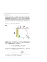
Example 20.3

(The Dipole Field Along the Dipole Axis)

A proton and an electron separated by 2 × 10−10 m form an electric dipole, see
Fig. 20.10. Use exact and approximate formulae to calculate the electric field on
the x-axis at a distance 20 × 10−10 m to the right of the dipole’s center.


670

20 Electric Fields

Electron

-e

Proton

-

0

-a

+e

E−

+

P

E+

x

+a
a = 10−10 m
20 × 10−10 m

Fig. 20.10

Solution: In this problem we have a = 10−10 m, q = e = 1.6 × 10−19 C, x =
20 × 10−10 m, ke = (9 × 109 N.m2 /C2 ) (1.6 × 10−19 C) = 1.44 × 10−9 N.m2 /C,
x − a = 19 × 10−10 m, and x + a = 21 × 10−10 m. Using the exact formula given
by Eq. 20.11 in the case of x > +a, we have:
E = ke

1
1
−
(x − a)2
(x + a)2

= (1.44 × 10−9 N.m2 /C)

1
1
−
(19 × 10−10 m)2

(21 × 10−10 m)2

= (1.44 × 10−9 N.m2 /C)[2.770 × 1017 m−2 − 2.268 × 1017 m−2 ]
= 7.236 × 107 N/C
On the other hand, we have x

a and we can use the approximate formula given

by Eq. 20.13 as follows:
2a e
4a
p
= 2k 3 = ke 3
3
x
x
x
(4 × 10−10 m)
= (1.44 × 10−9 N.m2 /C)
(20 × 10−10 m)3

E = 2k

= 7.200 × 107 N/C
Clearly this calculation is a good approximation when x/a = 20.

20.4

Electric Field of a Continuous Charge Distribution

The electric field at point P due to a continuous charge distribution shown in Fig. 20.11
can be evaluated by:
(1) Dividing the charge distribution into small elements, each of charge
located relative to point P by the position vector →
r =r →
rˆ .
n

n n

qn that is


20.4 Electric Field of a Continuous Charge Distribution
→

En due to the nth element as follows:

(2) Using Eq. 20.4 to evaluate the electric field
→

En = k

671

qn →
rˆn
rn2

(20.18)

(3) Evaluating the order of the total electric field at P due to the charge distribution
by the vector sum of all the charge elements as follows:
→

qn →
rˆn
rn2

E ≈k
n

(20.19)

(4) Evaluating the total electric field at P due to the continuous charge distribution
in the limit qn → 0 as follows:
→

E = k lim

qn →0

n

qn →
rˆn = k
rn2

dq →
rˆ

r2

(20.20)

where the integration is done over the entire charge distribution.
Fig. 20.11 The electric field

P

→

E at point P due to a
continuous charge distribution

qn

is the vector sum of all the
fields

→

En

rn

En (n = 1, 2, · · · ) due

to the charge elements
qn (n = 1, 2, · · · ) of the
charge distribution

Now we consider cases were the total charge is uniformly distributed on a line,
on a surface, or throughout a volume. It is convenient to introduce the charge density
as follows:
(1) When the charge Q is uniformly distributed along a line of length L, the linear
charge density λ is defined as:
λ=

Q
L

(20.21)

where λ has the units of coulomb per meter (C/m).
(2) When the charge Q is uniformly distributed on a surface of area A, the surface
charge density σ is defined as:


672

20 Electric Fields

σ =

Q
A

(20.22)

where σ has the units of coulomb per square meter (C/m2 ).

(3) When the charge Q is uniformly distributed throughout a volume V, the volume
charge density ρ is defined as:
ρ=

Q
V

(20.23)

where ρ has the units of coulomb per cubic meter (C/m3 ).
Accordingly, the charge dq of a small length dL, a small surface of area dA, or a
small volume dV is respectively given by:
dq = λ dL, dq = σ dA, dq = ρ dV

(20.24)

20.4.1 The Electric Field Due to a Charged Rod
For a Point on the Extension of the Rod
Figure 20.12 shows a rod of length L with a uniform positive charge density λ
and total charge Q. In this figure, the rod lies along the x-axis and point P is taken to
be at the origin of this axis, located at a constant distance a from the left end. When
we consider a segment dx on the rod, the charge on this segment will be dq = λ dx.

y
P

dx

x

E

+ + + + + + + + + + + +
dq

0

a

x

L
→

Fig. 20.12 The electric field E at point P due to a uniformly charged rod lying along the x-axis. The
magnitude of the field due to a segment of charge dq at a distance x from P is k dq/x 2 . The total field is
the vector sum of all the segments of the rod
→

The electric field dE at P due to this segment is in the negative x direction and
has a magnitude given by: