Hafez a radi, john o rasmussen auth principles of physics for scientists and engineers 2 28

20.4 Electric Field of a Continuous Charge Distribution

dE = k

673

dq
λ dx
=k 2
2
x
x

(20.25)

The total electric field at P due to all the segments of the rod is given by Eq. 20.20
after integrating from one end of the rod (x = a) to the other (x = a + L) as follows:
a+L

E=

dE =

k
a

λ dx
= kλ
x2

1

1
+
= kλ −
a+L a

a+L

x −2 dx = kλ − 1x

a+L
a

(20.26)

a

kλL
=
a(a + L)

When we use the fact that the total charge is Q = λL, we have:
E=

kQ
a(a + L)

(Toward the left)

If P is a very far point from the rod, i.e. a

(20.27)

L, then L can be neglected in the

denominator of Eq. 20.27. Accordingly, we have E ≈ kQ/a2 , which resembles the
magnitude of the electric field produced by a point charge.

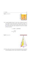
For a Point on the Perpendicular Bisector of the Rod
A rod of length L has a uniform positive charge density λ and total charge Q. The
rod is placed along the x-axis as shown in Fig. 20.13. Assume that point P is on
the perpendicular bisector of the rod and is located at a constant distance a from the
origin of the x-axis. The charge on a segment dx on the rod will be dq = λ dx.
Fig. 20.13 A rod of length L
has a uniform positive charge
density λ and an electric field
→

d E at point P due to a segment

y
dE

d Ey

d Ex

P

of charge dq, where P is
located along the

perpendicular bisector of the
rod. From symmetry, the total

a

r

dq

field will be along the y-axis

θ

θο

+ + + + + + + + + + + +
x
0
dx
L

x


674

20 Electric Fields
→

The electric field dE at P due to this segment has a magnitude:

dE = k

dq
λ dx
=k 2
2
r
r

(20.28)

This field has a vertical component dEy = dE sin θ along the y-axis and a horizontal
component dEx perpendicular to it, as shown in Fig. 20.13. An x-component at such
a location is canceled out by a similar but symmetric charge segment on the opposite
side of the rod. Thus:
Ex =

dEx = 0

(20.29)

The total electric field at P due to all segments of the rod is given by two times
the integration of the y-component from the middle of the rod (x = 0) to one of the
ends (x = L/2). Thus:
x=L/2

E=2

x=L/2

dEy = 2
x=0

x=L/2

dE sin θ = 2 k λ
x=0

x=0

sin θ dx
r2

(20.30)

To perform the integration of this expression, we must relate the variables θ, x, and
r. One approach is to express θ and r in terms of x. From the geometry of Fig. 20.13,
we have:
x 2 + a2 and sin θ =

r=

a
a
=√
2
r
x + a2

(20.31)

Therefore, Eq. 20.30 becomes:
L/2

E = 2 kλ a
0

dx
(x 2 + a2 )3/2

(20.32)

From the table of integrals in Appendix B, we find that:
(x 2

dx
x
=
2
3/2
+a )
a2 (x 2 + a2 )

(20.33)

Thus:
L/2

E = 2kλ a
0

= 2kλ a

x
dx
= 2 kλ a
√
2
2
3/2
(x + a )
a2 x 2 + a2
L/2

a2

(L/2)2

+ a2

−0 =

L/2
0

kλ L
a (L/2)2 + a2

(20.34)

20.4 Electric Field of a Continuous Charge Distribution

675

When we use the fact that the total charge is Q = λL, we have:
E=

kQ
a

a2

+ (L/2)2

or

When P is a very far point from the rod, a

E=

kλ L
a

a2

+ (L/2)2

(20.35)

L, we can neglect (L/2)2 in the denom-

inator of Eq. 20.35. Thus, E ≈ kQ/a2 . This is just the form of a point charge. For an
infinitely long rod we get:
2kλ

E = lim

L→∞

a (2a/L)2 + 1

⇒

E = 2k

λ
a

(20.36)

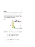
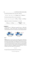
Example 20.4

Figure 20.14 shows a non-conducting rod that has a uniform positive charge
density +λ and a total charge Q along its right half, and a uniform negative
charge density −λ and a total charge −Q along its left half. What is the direction
and magnitude of the net electric field at point P that shown in Fig. 20.14?
Fig. 20.14

y

P

a
-Q

+Q

x
0

L

Solution: When we consider a segment dx on the right side of the rod, the charge
on this segment will be dq = λ dx, see Fig. 20.15.
→
The electric field dE + at P due to this segment is directed outwards and away
from the positive charge dq and has a magnitude:
dE+ = k

dq
λ dx
=k 2
r2
r

A symmetric segment on the opposite side of the rod, but with a negative charge,
→

creates an electric field dE − that is directed inwards and toward this segment and

676

20 Electric Fields
→

→

has the same magnitude as dE + , i.e. dE+ = dE− . The resultant electric field dE

from both symmetric segments will be a vector to the left, see Fig. 20.15, and its
magnitude will be given by:
dE = dE+ cos θ + dE+ cos θ = 2 dE+ cos θ
= 2k

λ dx x
= k λ(x 2 + a2 )−3/2 (2x)dx
r2 r

Fig. 20.15

d E+

y
P

dE
dE−

a

r

-Q

r

θ

dq

θ

x

+
0

x

+Q

dx

L
The total electric field at P due to all segments of the rod is found by integrating dE from x = 0 to only x = L/2,since the negative charge of the rod is
considered in evaluating dE. Thus:
x=L/2

E=

(x 2 + a2 )−3/2 (2x dx)

dE = k λ
x=0

To evaluate the integral in this equation, we transform it to the form
un du = un+1 /(n + 1), as we shall do in solving Eq. 20.53. Thus:
E=kλ
= 2k λ

(u2 + a2 )−1/2
−1/2
1
−
a

u=L/2

=kλ
u=0

−2
(L/2)2

+ a2

−

−2

a

1
(L/2)2 + a2

When we use the fact that the magnitude of the charge Q is given by Q = λL/2,
we get:


20.4 Electric Field of a Continuous Charge Distribution

E=

4k Q
L

1
−
a

677

1
(L/2)2 + a2

When P is very far away from the rod, i.e. a L, we can neglect (L/2)2 in
the denominator of this equation and hence get E ≈ 0. In this situation, the two
oppositely charged halves of the rod would appear to point P as if they were two
coinciding point charges and hence have a zero net charge.

Example 20.5

An infinite sheet of charge is lying on the xy-plane as shown in Fig. 20.16. A
positive charge is distributed uniformly over the plane of the sheet with a charge
per unit area σ. Calculate the electric field at a point P located a distance a from
the plane.

z

dE

dE z

dE x

P

+

+

a
+

r

+

o
+

y
x

+

θ

+

dx

+
x

Fig. 20.16


678

20 Electric Fields

Solution: Let us divide the plane into narrow strips parallel to the y-axis.
A strip of width dx can be considered as an infinitely long wire of charge per
unit length λ = σ dx. From Eq. 20.36, at point P, the strip sets up an electric field
→

dE lying in the xz-plane of magnitude:
dE = 2k

λ
σ dx
= 2k
r
r
→

→

This electric field vector can be resolved into two components dE x and dE z .
→
By symmetry the components dE x will sum to zero when we consider the entire
sheet of charge. Therefore, the resultant electric field at point P will be in the
z-direction, perpendicular to the sheet. From Fig. 20.16, we find the following:
dEz = dE sin θ

and hence:

+∞

E=

dEz = 2kσ
−∞

sin θ dx
r

To perform the integration of this expression, we must first relate the variables θ,
x, and r. One approach is to express θ and r in terms of x. From the geometry of

Fig. 20.16, we have:
r=

x 2 + a2 and sin θ =

a
a
=√
2
r
x + a2

Then, from the table of integrals in Appendix B, we find that:
+∞

E = 2kσ a
−∞

1
dx
x
= 2kσ a tan−1
x 2 + a2
a
a

= 2kσ tan−1 (∞) − tan−1 (−∞) = 2kσ

+∞
−∞

π
π
+
2
2

Thus:
E = 2π kσ =

σ
2 ◦

This result is identical to the one we shall find in Sect. 20.4.4 for a charged
disk of infinite radius. We note that the distance a from the plane to the point P
does not appear in the final result of E. This means that the electric field set up at
any point by an infinite plane sheet of charge is independent of how far the point


20.4 Electric Field of a Continuous Charge Distribution

679

is from the plane. In other words, the electric field is uniform and normal to the
plane.
Also, the same result is obtained if the point P lies below the xy-plane. That
is, the field below the plan has the same magnitude as that above the plane but as
a vector it points in the opposite direction.

20.4.2 The Electric Field of a Uniformly Charged Arc

Assume that a rod has a uniformly distributed total positive charge Q. Also assume
that the rod is bent into a circular section of radius R and central angle φ rad. To find
the electric field at the center P of this arc, we place coordinate axes such that the
axis of symmetry of the arc lies along the y-axis and the origin is at the arc’s center,
see Fig. 20.17a. If we let λ represent the linear charge density of this arc which has
a length Rφ, then:
λ=

Q
Rφ

(20.37)

For an arc element ds subtending an angle dθ at P, we have:
ds = R dθ

(20.38)

Therefore, the charge dq on this arc element will be given by:
dq = λ ds =

Q
Q
R dθ = dθ
Rφ
φ

(20.39)

To find the electric field at point P, we first calculate the magnitude of the electric

field dE at P due to this element of charge dq, see Fig. 20.17b, as follows:
dE = k

dq
kQ
= 2 dθ
2
R
R φ

(20.40)

This field has a vertical component dEy = dE cos θ along the y-axis and a horizontal
component dEx along the negative x-axis, as shown in Fig. 20.17b. The x-component
created at P by any charge element dq is canceled by a symmetric charge element on
the opposite side of the arc. Thus, the perpendicular components of all of the charge
elements sum to zero. The vertical component will take the form:
dEy = dE cos θ =

kQ
cos θ dθ
R2 φ

(20.41)


680

20 Electric Fields

Consequently, the total electric field at P due to all elements of the arc is given by
the integration of the y-component as follows:
E=

dEy =

kQ
R2 φ

+φ/2

cos θ dθ =
−φ/2

kQ
sin θ
R2 φ

+φ/2
−φ/2

=

φ
kQ
φ
sin − sin −
R2 φ
2
2

(20.42)

y

y

dE
P

dE y
P

x

φ

dθ

θ

R

R

x

dE x

dq

R
Q

Q

R

ds

s
(b)

(a)

Fig. 20.17 (a) A circular arc of radius R, central angle φ, and center P has a uniformly distributed
→

positive charge Q. (b) The figure shows the electric field d E at P due to an arc element ds having a charge
dq. From symmetry, the horizontal components of all elements cancel out and the total field is along the
y-axis

Finally, the total electric field at P will be along the y-axis and will have a magnitude given by:
E=

kQ sin φ/2
R2 φ/2

(20.43)

There are three special cases to Eq. 20.43:

(1) φ = 0 (Point charge)
When we apply the limiting case lim [sin(φ/2)/(φ/2)] = 1,we get:
φ →0

E=

kQ
R2

(20.44)


20.4 Electric Field of a Continuous Charge Distribution

681

(2) φ = π (Half a circle of radius R)
When we substitute with sin(π/2)/(π/2) = 2/π, we get:
E=

2kQ
π R2

(20.45)

(3) φ = 2π (A ring of radius R)
When we substitute with sin π = 0, we get:
E=0

(20.46)

This is an expected result, since we shall see that Eq. 20.50 gives E = 0 when P
is at the center of the ring, i.e. when a = 0.

20.4.3 The Electric Field of a Uniformly Charged Ring
Assume that a ring of radius R has a uniformly distributed total positive charge Q,
see Fig. 20.18. Also, assume there is a point P that lies at a distance a from the center
of the ring along its central perpendicular axis, as shown in the same figure.
Fig. 20.18 A ring of radius R

z
dE

having a uniformly distributed

dEz

positive charge Q. The figure
→

shows the electric field d E at

d E⊥

an axial point P due to a

P

segment of charge dq. The

θ

horizontal components will
cancel each other, and the total

Q

a

r

field will be along the z-axis

R

dq

To find the electric field at P, we first calculate the magnitude of the electric field
dE at P due to this segment of charge dq as follows:


682

20 Electric Fields

dE = k

dq
r2

(20.47)

This field has a vertical component dEz = dE sin θ along the z-axis and a component
dE⊥ perpendicular to it, as shown in Fig. 20.18. The perpendicular component created
at P by any charge segment is canceled by a symmetric charge segment on the opposite
side of the ring. Thus, the perpendicular components of all of the charge segments
√
sum to zero. Using r = R2 + a2 and sin θ = a/r, the vertical component will take
the form:
dEz = dE sin θ = k

dq a
ka dq
= 2
r2 r
(R + a2 )3/2

(20.48)

The total electric field at P due to all segments of the ring is given by the integration
of the z-component as follows:
E=
=

dEz =

(R2

ka
(R2 + a2 )3/2

ka dq
+ a2 )3/2

(20.49)

dq

Since dq represents the total charge Q over the entire ring, then the total electric
field at P will be given by:
E=

(R2

kQa
+ a2 )3/2

(20.50)

This formula shows that the field is zero at the center of the ring, i.e., at a = 0.When
point P is very far from the ring, i.e., a R, then we can neglect R2 in the denominator
of Eq. 20.50 and get E ≈ kQ/a2 . This form resembles the one we got for a point
charge.

20.4.4 The Electric Field of a Uniformly Charged Disk
Assume that a disk of radius R has a uniform positive surface-charge density σ. Also,
assume that a point P lies at a distance a from the disk along its central perpendicular
axis, see Fig. 20.19.
To find the electric field at P, we divide the disk into concentric rings, then calculate
the electric field at P for each ring by using Eq. 20.50, and finally we can sum up the

contributions of all the rings.


20.4 Electric Field of a Continuous Charge Distribution

683

Fig. 20.19 A disk of radius R

z

has a uniform positive surface

E

charge density σ. The ring
shown has a radius r and radial

P

width dr. The total electric
field at an axial point P is

Ring

Charge per
unit area σ

a

directed along this axis

Disk

dr
R

r

Figure 20.19 shows one such ring, with radius r, radial width dr, and surface area
dA = 2π r dr. Since σ is the charge per unit area, then the charge dq on this ring is:
dq = σ dA = 2π rσ dr

(20.51)

Using this relation in Eq. 20.50, and replacing E with dE, R with r, and Q with
dq = 2π rσ dr, then we can calculate the field resulting from this ring as follows:
dE =

(r 2

2r dr
ka
(2π rσ dr) = π kσ a 2
2
3/2
+a )
(r + a2 )3/2

(20.52)

To find the total electric field, we integrate this expression with respect to the
variable r from r = 0 to r = R. This gives:
R

E=

(r 2 + a2 )−3/2 (2r dr)

dE = π kσ a

(20.53)

0

un du = un+1 /(n + 1) by setting

To solve this integral, we transform it to the form
u=

r2

+ a2 ,

and du = 2r dr. Thus, Eq. 20.53 becomes:
u=R2 +a2

R
2 −3/2

(r + a )

E = π kσ a

2

(2r)dr = π kσ a

0

= π kσ a

u=a2

u=R2 + a2
u−1/2

−1/2

u−3/2 du

u= a2

= π kσ a

(R2

+ a2 )−1/2
−1/2

(20.54)
−

a−1
−1/2


684

20 Electric Fields

Rearranging the terms, we find:
E = 2π kσ 1 − √

a
R2

+ a2

(20.55)

Using k = 1/4π ◦ , where ◦ is the permittivity of free space, it is sometimes preferable to write this relation as:
E=

a
σ
1− √
2
2 ◦
R + a2

(20.56)

We can calculate the field when point P is very close to the disk (the near-field
approximation) by assuming that R a, or by assuming the disk to be an infinite
sheet when R → ∞ while keeping a finite. In both cases, the second term between
the two brackets of Eq. 20.56 approaches zero, and the equation is reduced to:
⎫
⎧
⎪
⎪
(Points
very
close
to
the
disk)
⎪
⎪
⎬
⎨
σ
(20.57)
E=
or
⎪
2 ◦ ⎪
⎪
⎪
⎭

⎩
(Infinite sheet)

20.5

Electric Field Lines

The concept of electric field lines was introduced by Faraday as an approach to help
us visualize electric fields.
Spotlight
An electric field line is an imaginary line drawn in such a way that the direction
of its tangent at any point is the same as the direction of the electric field vector
→

E at that point, see Fig. 20.20.

Since the direction of an electric field generally varies from one point to another, the
electric field lines are usually drawn as curves, see Fig. 20.20.


20.5 Electric Field Lines

685

Fig. 20.20 The direction of

Electric field at
point Q

the electric field at any point is

the tangent to the electric field

Q

line at this point

Electric field
at point P
Electric field line

P

The relation between electric field lines and electric field vectors is as follows:
Spotlight
→

• The electric field vector E is tangent to the electric field line at any point.
• The direction of the electric field line at any point is the same as the
direction of the electric field.
• The number of electric field lines per unit area, measured in the plane of
→
the lines, is proportional to the magnitude of E . Thus, the electric field
lines are closer together when the electric field is strong, and far apart
when the field is weak.

The rules for drawing electric field lines are as follows:
Spotlight
• Electric field lines must emerge from a positive charge and end on a negative charge. For a system that has an excess of one type of charge, some
lines will emerge or end infinitely far away.
• The number of lines emerging from a positive charge or ending at a negative

charge is proportional to the magnitude of the charge.
• Electric field lines cannot cross each other.

The above rules are used in the six cases shown in Fig. 20.21.


686

20 Electric Fields

−q

q

E

E

(a)

q

(b)
−q

q
N

N

Neutral point

(c)
−q

−q

(d)

q

(e)

(f)

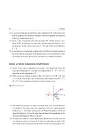
Fig. 20.21 The figure shows the electric field lines of: (a) a positive point charge, (b) a negative point
charge, (c) two equal positive charges, (d) two equal negative charges, (e) an electric dipole, and (f) a side
view of an infinite sheet of charge

20.6

Motion of Charged Particles in a Uniform Electric Field

When a particle of charge q and mass m is in an external electric field of strength
→
→
→
E , a force qE will be exerted on this particle. If qE is the only acting force on the
→

particle, then according to Newton’s second law, F = m→
a , the acceleration of the
particle will be given by:
→

→

a = qE /m

→

If E is uniform, then →
a will be constant vector.

(20.58)


20.6 Motion of Charged Particles in a Uniform Electric Field

687

Motion of a Charged Particle Along an Electric Field
Consider a particle of positive charge q and mass m in a uniform horizontal electric
→

field E produced by two charged plates that are separated by a distance d as shown
in Fig. 20.22.
→

If the particle is released from rest at the positive plate and qE is the only force

that acts on the particle, then the particle will move horizontally along the x-axis with
→

an acceleration →
a = qE /m. In such a case, we can apply the kinematics equations
(see Chap. 3) on the initial and final motion as follows:
• The particle’s time of flight t:
x = v◦ t + 21 a t 2

⇒

d =0+

1
2

qE 2
t
m

t=

2md
qE

(20.59)

v=

2qEd

m

(20.60)

⇒

• The speed of the particle v:
v = v◦ + a t

⇒

v =0+

qE
m

2md
qE

⇒

• The kinetic energy of the particle K:
K = 21 mv 2

⇒

K = qEd

(20.61)

The last result can also be obtained from the application of the work-energy theorem
W = K because W = (qE)d and K = Kf − Ki = K.

Example 20.6

In Fig. 20.22, assume that the charged particle is a proton of charge q = +e. The
proton is released from rest at the positive plate. In this case, each of the two
oppositely charged plates which are d = 2 cm apart has a charge per unit area of
σ = 5 μC/m2 . (a) What is the magnitude of the electric field between the two
plates? (b) What is the speed of the proton as it strikes the second plate?
Solution: (a) The electric field arises from two infinite plates, Thus:
E=

σ
σ
5 × 10−6 C/m2
σ
+
=
=
= 5.65 × 105 N/C
2 ◦
2 ◦
8.85 × 10−12 C/N.m2
◦


688

20 Electric Fields

→

Fig. 20.22 A force qE

E

exerted on a positive charge q
→

by a uniform electric field E

°= 0

established between two
oppositely charged plates

v

qE

qE

t =0

t

d

(b) We first find the proton’s acceleration from Newton’s second law:
a=

eE
(1.6 × 10−19 C)(5.65 × 105 N/C)
F
=
=
= 5.41 × 1013 m/s2
m
m
1.67 × 10−27 kg

Then, using x = v◦ t + 21 a t 2 , we find that d = 21 a t 2 . Thus:
t=

2d
=
a

2(0.02 m)
= 2.72 × 10−8 s
5.41 × 1013 m/s2

Finally, we use v = v◦ + a t to find the speed of the proton as follows:
v = a t = (5.41 × 1013 m/s2 )(2.72 × 10−8 s) = 1.47 × 106 m/s

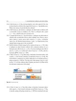
Motion of a Charged Particle Perpendicular to an Electric Field
Consider an electron of charge q = −e and mass m being projected in a uniform
→
vertical electric field E that is established in a region of length L by two oppositely
charged plates as shown in Fig. 20.23. If the initial speed v◦ of the electron at t = 0

→

is along the nagative x-axis, and if E is along the y-axis, then the acceleration of the
electron will be constant along the positive y-axis (ignoring the gravitational force
and assuming vacuum conditions). That is:
ax = 0 ay =

eE
(Upwards)
m

(20.62)

When we apply the kinematics equations with vx◦ = v◦ and vy◦ = 0 while the electron
is in the region of the electric field, we find that:


20.6 Motion of Charged Particles in a Uniform Electric Field

689

The components of the electron’s velocity at time t will be:
vx = vx◦ = v◦
eE
t
vy = ay t =
m

Along x
Along y

(20.63)

The components of the electron’s position at time t will be:
Along x

x = v◦ t

Along y

y = 21 ay t 2 =

y

−e -

-

t1

y2

-

E

t=0

(20.64)

eE 2
t
2m

°

h

α
y1

D

y1
x

L

D
→

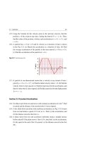
Fig. 20.23 The effect of an upward force −eE exerted on an electron projected horizontally with speed
→

v◦ into a downward uniform electric field E

The electron will move a distance L horizontally and a distance y1 vertically before
leaving the region of the electric field, see Fig. 20.23. According to Eq. 20.64, the
time at this instant will be:
t1 =

L
v◦

(20.65)

The vertical position y1 that corresponds to this time is:
y1 =

eEL 2
2mv◦2

(20.66)


690

20 Electric Fields

When the electron leaves the region of the electric field, with vx = v◦ and
vy = ay t1 , the electric force vanishes and the electron continues to move in a straight
line with a constant velocity:
→

v→ = v◦ i +

eEL →
j
mv◦

(20.67)

This velocity makes an angle α with the horizontal and so:
tan α =

eEL
eEL/mv◦
=
v◦
mv◦2

(20.68)

The extra vertical distance y2 that the electron will move before hitting the screen,
which is located at a horizontal distance D from the plates, is given by:
y2 = D tan α = D

eEL
mv◦2

(20.69)

Finally, the total vertical distance h that the electron will move is:
h = y1 + y2 =

eEL
mv◦2

L
+D

2

(20.70)

Example 20.7

In Fig. 20.23, assume that the horizontal length L of the plates is 5 cm, and assume
that the separation D between the plates and the screen is 50 cm. If the uniform
electric field has E = 250 N/C, and the electron’s initial speed v◦ is 2 × 106 m/s,
then; (a) What is the acceleration of the electron between the two plates? (b) Find
the time when the electron leaves the two plates. (c) Find the electron’s vertical
position before leaving the field region. (d) Find the electron’s vertical distance
before hitting the screen.
Solution: (a) Using the magnitude of the electronic charge e = 1.6 × 10−19 C and
the electronic mass m = 9.11 × 10−31 kg in Eq. 20.62, we get:
ax = 0 and ay =

eE (1.6 × 10−19 C)(250 N/C)
=
= 4.391 × 1013 m/s2
m
9.11 × 10−31 kg


20.6 Motion of Charged Particles in a Uniform Electric Field

691

(b) Using Eq. 20.65 for the horizontal motion, we get:
t1 =

L
0.05 m
= 2.5 × 10−8 s
=
v◦
2 × 106 m/s

(c) Using Eq. 20.66 for the vertical motion, we get:
y1 =

eEL 2 (1.6 × 10−19 C)(250 N/C)(0.05 m)2
=
= 0.0137 m = 1.37 cm
2mv◦2
2(9.11 × 10−31 kg)(2 × 106 m/s)2

Alternatively, we can use Eq. 20.64 to find y1 as follows:
y1 = 21 ay t12 = 21 (4.391 × 1013 m/s2 )(2.5 × 10−8 s)2 = 0.0137 m = 1.37 cm
(d) We calculate y2 from Eq. 20.69 as follows:
y2 = D

eEL (0.5 m)(1.6 × 10−19 C)(250N/C)(0.05 m)
=
= 0.274 m = 27.4 cm
mv◦2
(9.11 × 10−31 kg)(2 × 106 m/s)2

Therefore, the total vertical distance moved by the electron is:
h = y1 + y2 = 0.0137 m + 0.274 m = 0.2877 m = 28.77 cm

20.7

Exercises

Section 20.2 Electric Field of a Point Charge
(1) Find the electric field of a 1 μC point charge at a distance of: (a) 1 cm, (b) 1 m,
and (c) 1 km.
(2) Find the value of a point charge if it has an electric field of 1 N/C at points:
(a) 1 cm away, (b) 1 m away, and (c) 1 km away.
(3) A vertical electric field is set up in space to compensate for the gravitational
force on a point charge. What is the required magnitude and direction of the
field when the point charge is: (a) an electron? (b) a proton? Comment on the
obtained values.
(4) An electron experiences a force of 8 × 10−14 N directed toward the front side
of a TV tube (the positive x-direction). (a) What is the magnitude and direction
of the electric field that produces this force? (b) What is the magnitude of the
acceleration of the electron?


692

20 Electric Fields

(5) A 4 μC point charge is placed at a point P(x = 0.2 m, y = 0.4 m). What is the
→

electric field E due to this charge: (a) at the origin, (b) at x = 1 m and y = 1 m.
(6) Two point charges q1 = +9 μC and q2 = −4 μC are separated by a distance
L = 10 cm, see Fig. 20.24. Find the point at which the resultant electric field is

zero.

Fig. 20.24 See Exercise (6)

q1

q2

+

L

(7) Three negative point charges are placed at the vertices of an isosceles triangle as shown in Fig. 20.25. Given that a = 10 cm, q1 = q3 = −2 μC, and q2 =
−4 μC, find the magnitude and direction of the electric field at point P (which
is midway between q1 and q3 ).
Fig. 20.25 See Exercise (7)

q1

a
q2

P

a

q3

(8) Four charges of equal magnitude are located at the four corners of a square
of side a = 0.1 m. Find the magnitude and direction of the electric field at

the center P of the square if: (a) all the charges are positive, i.e. qi = 5 μC,
where i = 1, 2, 3, 4, see top of Fig. 20.26. (b) the charges alternate in sign
around the perimeter of the square, i.e. q1 = q3 = 5 μC and q2 = q4 = −5 μC,
see middle of Fig. 20.26. (c) the anti-clockwise sequence of the charge signs
around the perimeter are plus, plus, minus, and minus, i.e. q1 = q2 = 5 μC and
q3 = q4 = −5 μC, see lower of Fig. 20.26.