Hafez a radi, john o rasmussen auth principles of physics for scientists and engineers 2 29

20.7 Exercises
Fig. 20.26 See Exercise (8)

693

y

q1

a

q4
x

P

q2

q3

a
y

q1

a

q4
x

P

q2

q3

a
y

q1

a

q4
x

P

q2

q3

a

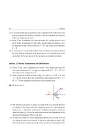
Section 20.3 Electric Field of an Electric Dipole
(9) Two point charges q1 = −6 μC and q2 = +6 μC are placed at two vertices of
an equilateral triangle, see Fig. 20.27. If a = 10 cm, find the electric field at the
third corner.
Fig. 20.27 See Exercise (9)

a

a

q1

a

q2

(10) A proton and an electron form an electric dipole and are separated by
a distance of 2a = 2 × 10−10 m, see Fig. 20.28. (a) Use exact formulas to
calculate the electric field along the x-axis at x = −10a, x = −2a, x = −a/2,


694

20 Electric Fields

x = +a/2, x = +2a, and x = +10a. (b) Show that at both points x = ±10a, the
approximate formula given by Eq. 20.13 has a very close percentage difference
from the exact value.
Fig. 20.28 See Exercise (10)

-e

Electron

y

Proton

+e
x

-a

0

a = 10− 10 m

+a

(11) Rework the calculations of Exercise 10 but on the y-axis at y = −10 a,
y = −2 a, y = −a/2, y = +a/2, y = +2a, and y = +10a. In part (b), use
Eq. 20.17.

Section 20.4 Electric Field of a Continuous Charge Distribution
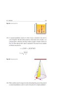
(12) A non-conductive rod of length L has a total negative charge −Q that is uniformly distributed along its length, see Fig. 20.29. (a) Find the linear charge
density of the rod. (b) Use the coordinates depicted in the figure to prove that the
electric field at point P, a distance a from the right end of the rod, has the same
form as the one given by Eq. 20.27. (c) When P is very far from the rod, i.e.
a L, show that the electric field reduces to the electric field of a point charge
(i.e. the rod would look like a point charge). (d) If L = 15 cm, Q = 25 μC, and
a = 20 cm, find the value of the electric field at P.

y
−Q

P

x

0

L

a

Fig. 20.29 See Exercise (12)

(13) A non-conductive rod lies along the x-axis with one of its ends located at x = a
and the other end located at ∞, see Fig. 20.30. Starting from the definition of
an electric field of a differential element on the rod, find the electric field at the


20.7 Exercises

695

origin if: (a) the rod carries a uniform positive linear charge density λ. (b) the
rod carries a positive varying linear charge density λ = λ◦ a/x.

y

λ

-x
0

∞

a

Fig. 20.30 See Exercise (13)

(14) A uniformly charged ring of radius 15 cm has a total charge of 50 μC. Find the
electric field on the central perpendicular axis of the ring at: (a) 0 cm, (b) 1 cm,
(c) 10 cm, and (d) 100 cm. (e) What do you observe about the values you just
calculated?
(15) A charged ring of radius R = 0.5 m has a gap d = 0.1 m, see Fig. 20.31.
Calculate the electric field at its center C if it carries a uniform charge q = 1 μC.

Fig. 20.31 See Exercise (15)

q=1

C

C

d = 0. 1m

R = 0. 5 m

(16) Figure 20.32 shows a non-conductive semicircular arc of radius R that consists
of two quarters. The semicircle has a uniform positive total charge Q along its
right half, and a uniform negative total charge −Q along its left half. Find the
resultant electric field at the center of the semicircle.
Fig. 20.32 See Exercise (16)

-Q

P

R

+Q
R

R


696

20 Electric Fields

(17) Two non-conductive semicircular arcs, one of a uniform positive charge +Q
and the other of a uniform negative charge −Q, form a circle of radius R,
see Fig. 20.33. Find the resultant electric field at the center of the circle, and
compare it with the result of Exercise 16.
Fig. 20.33 See Exercise (17)

-Q

+Q

P

R
R

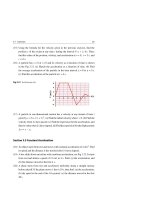
(18) If you consider a uniformly charged ring of total charge Q and a fixed radius
R (as in Fig. 20.18), then the graph of Fig. 20.34 would map the electric field
along the axis of such a ring as a function of z/R. Show that the maximum
√
√
electric field is Emax = 2k Q/3 3R2 and occurs at z = R/ 2.
Fig. 20.34 See Exercise (18)

E max

E

0

2

4

6

8

10

z /R

(19) An electron is constrained to move along the central axis of a ring of radius R
that has a uniform positive charge q, see Fig. 20.35. Show that when the position
x of the electron is much less than the radius R (x R), the electrostatic force

exerted on the electron can cause it to oscillate through the center of the ring
with an angular frequency given by ω = kqe/mR3 , where e and m are the
electronic charge and mass, respectively.
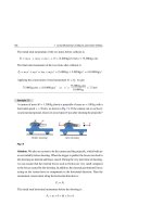
(20) Two non-conductive rings having the same radius R are arranged with their
central axes along a common horizontal line and separated by a distance of 4 R,
see Fig. 20.36. Ring 1 has a uniform positive charge q1 , while ring 2 has a
uniform positive charge q2 . Given that the net electric field is zero at point P,
which is at a distance R from ring 1 and on the common central axis of the
two rings, (a) find the ratio between the two charges. (b) If only the sign of q1


20.7 Exercises

697

is reversed, is it possible to have a point on the common axis where the net
electric field is zero? If so, where would it be?

q

Fig. 20.35 See Exercise (19)

x

R

0

-x

-e
F

R

x

x
Fig. 20.36 See Exercise (20)

Ring 2

Ring 1

q1

q2
C1

C2

P

R

R

R

4R

(21) A disk of radius R = 5 cm has a surface charge density σ = 6 μC/m2 on its
surface. Calculate the magnitude of the electric field at points on the central
axis of the disk located at: (a) 1 mm, (b) 1 cm, (c) 10 cm, and (d) 100 cm.
(22) A disk of radius R has a charge Q that is uniformly distributed over its surface
area. Show that Eq. 20.55 transforms to:
E=
Show that when a
formula:

2kQ
a
1− √
2
2
R
R + a2

R, the electric field approaches that of a point charge

E≈k

Q
(a
a2

R)

You may use the binomial expansion (1 + δ)p ≈ 1 + pδ when δ 1.
(23) Compare the obtained results of Exercise 21 to the near-field approximation

E = σ/2 ◦ as well as to the point charge approximation E = k(π R2 σ )/a2 , and
find which result(s) of Exercise 21 match the two approximations.


698

20 Electric Fields

(24) A disk of radius R has a surface charge density σ and an electric field of magnitude E◦ = σ/2 ◦ at the center of its surface, see Fig. 20.37. At what distance
z along the central axis of the disk is the magnitude of the electric field E equal
to one-half of E◦?
Fig. 20.37 See Exercise (24)

E

σ
4

E0

Charge per
unit area σ

°

σ
2

z
°

0

R

(25) Find the electric field between two oppositely-charged infinite sheets of charge,
each having the same charge magnitude and surface charge density σ, but
opposite signs, see Fig. 20.38.

+

Fig. 20.38 See Exercise (25)

+
E

+
+

Section 20.5 Electric Field Lines
(26) (a) A negatively charged disk has a uniform charge per unit area. Sketch the
electric field lines in the plane of the plane of the disk passing through its center.
(b) Redo part (a) taking the disk to be positively charged. (c) A negatively
charged rod has a uniform charge per unit length. Sketch the electric field
lines in the plane of the rod. (d) Three equal positive charges are placed at the
corners of an equilateral triangle. Sketch the electric field lines in the plane
of the charges. (e) An infinite linear rod has a uniform charge per unit length.
Sketch the electric field lines in the plane of the rod.

20.7 Exercises

699

Section 20.6 Motion of Charged Particles in a Uniform Electric Field
(27) An electron and a proton are released simultaneously from rest in a uniform
electric field of 105 N/C. Ignore the effect of the fields of the electron and proton
on each other. (a) Find the speed and kinetic energy of the electron 50 ns after
it has been released. (b) Repeat part (a) for the proton.
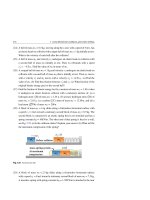
(28) Figure 20.39 shows two oppositely charged parallel plates that are separated
by a distance d = 1.5 cm. Each plate has a charge per unit area of magnitude
σ = 4 μC/m2 . An electron is released from rest at t = 0 from the negative plate.
(a) Calculate the electric field between the two plates. (b) Ignoring the effect of
gravity, find the resultant force exerted on the electron? (c) Find the acceleration
of the electron. (d) How long does it take the electron to strike the positive plate?
(e) What is the speed and kinetic energy of the electron just before striking the
positive plate?
+

Fig. 20.39 See Exercise (28)

E

+

t

° 0

+

-

t 0

-

+
d

(29) In Exercise 28 assume that the electron is projected from the positive plate
toward the negative plate with an initial speed v◦ at time t = 0. The electron
travels the distance d = 1.5 cm between the two plates and stops temporarily
before hitting the negatively charged plate. (a) Find the magnitude and direction
of its acceleration. (b) Find the value of the electron’s initial speed. (c) Find the
time before the electron stops temporarily.
(30) Two oppositely charged horizontal plates are separated by a distance d = 1 cm
and each has a length L = 3 cm, see Fig. 20.40. The electric field between the
plates is uniform and has a magnitude E = 102 N/m. An electron is projected
between the plates with a horizontal initial speed of v◦ = 106 m/s as shown.
Assuming this experiment is conducted in a vacuum, where will the electron
strike the upper plate?
(31) Repeat Exercise 30 when a proton replaces the electron.


700

20 Electric Fields

Fig. 20.40 See Exercise (30)

y

-

+

+

+

+

+
t 0

d/2

e-

°

x

x

E

L
(32) To prevent the Electron in exercise 30 from striking the upper plate, its initial

horizontal speed is increased to v◦ = 2 × 106 m/s, see Fig. 20.41, and it then
strikes a screen at a distance D = 30 cm. (a) What is the acceleration of the
electron in the region between the two plates? (b) Find the time when the
electron leaves the two plates. (c) What is the vertical position of the electron
just before leaving the region between the two plates? (d) Find the electron’s
total vertical distance just before hitting the screen.

y

y2

+

+

+

t 0

+

+

d/ 2

-

t1

-

E

e-

y1

D

h

y1
x

L

D

Fig. 20.41 See Exercise (32)

(33) Repeat Exercise 32 when a proton replaces the electron.


21

Gauss’s Law

Although Coulomb’s law is the governing law in electrostatics, its form does not
always simplify calculations in situations involving symmetry. In this chapter, we
introduce Gauss’s law as an alternative method for calculating electric fields of certain

highly symmetrical charge distribution systems. In addition to being simpler than
Coulomb’s law, Gauss’s law permits us to use qualitative reasoning.

21.1

Electric Flux
→

Consider a uniform electric field E penetrating a small area A oriented perpendicularly to the field as shown in Fig. 21.1. Recall from Sect. 20.5 that the number of
electric field lines per unit area (measured in a plane perpendicular to the lines) is
→

proportional to the magnitude of E . Therefore, the total number of lines penetrating
the surface is proportional to EA. This product is called the electric flux1 E . Thus:
E

The SI units for

E

= EA

(21.1)

is newton-meters square per coulomb (N.m2 /C).

Spotlight
Electric flux is proportional to the number of electric field lines penetrating a
certain area.
→

If the area in Fig. 21.1 is tilted by an angle θ with respect to E, the flux through
it (the number of electric lines) will decrease. To visualize this, Fig. 21.2 shows an
1

The word “flux” comes from the Latin word meaning “to flow”.

H. A. Radi and J. O. Rasmussen, Principles of Physics,
Undergraduate Lecture Notes in Physics, DOI: 10.1007/978-3-642-23026-4_21,
© Springer-Verlag Berlin Heidelberg 2013

701


702

21 Gauss’s Law

area A that makes an angle θ with the field. The number of lines that cross the area
→

A is equal to the number that cross the area A , which is perpendicular to E and
hence A = A cos θ. Thus, the flux through A, E (A), is equal to the flux through A ,
E (A

). But according to Eq. 21.1, the flux through A is defined as
Therefore, the flux through A is:
E (A)

=

E (A

E (A

) = EA = EA cos θ

Area A

) = EA .

(21.2)

Side view
E
Area A

E

→

Fig. 21.1 Electric field lines representing a uniform electric field E that penetrates an area A perpendicularly (shown both in 3D and as a side view). The electric flux

E through this area is EA

E
Normal
θ

Area A

θ

Area A'

Area A'

θ

E

Area A

Side view
→

Fig. 21.2 Electric field lines representing a uniform electric field E penetrating an area A that is at an
angle θ with the field (both three dimensional and side views are displayed). Since the flux through A is
the same as through A , the flux through A is

E = EA cos θ

→

If we define a vector area A whose magnitude represents the surface area and
whose direction is defined to be perpendicular to the surface area as in Fig. 21.3, then
Eq. 21.2 can be written as:
→

E

→

= E • A = EA cos θ

(21.3)

The flux through a surface of area A has a maximum value EA when the surface is
perpendicular to the field (i.e. when θ = 0◦ ), and is zero when the surface is parallel
to the field (i.e. when θ = 90◦ ).


21.1 Electric Flux

703

A

Area A

A

θ

θ

E

Area A

E

Side view
→

Fig. 21.3 The definition of a vector area A whose magnitude represents the surface area and whose
direction is defined to be perpendicular to the surface area

Generally, the electric field may vary over the surface of any shape. Let us consider
the general surface depicted by the shape in Fig. 21.4 and calculate the electric flux
over the whole surface.

dA

θ

E

→

Fig. 21.4 The differential surface vector area d A of magnitude dA and direction perpendicular to the
→

differential surface area and pointing outwards. When the electric field E makes an angle θ with that
→

→

differential surface area, the differential flux d E is E • d A

→

We start by considering a differential vector surface area dA to be normal to the
surface and to point outwards at a specific location. If the electric field vector at this
→
location is E , then the differential electric flux d E through this differential area
will be:
→

d

E

→

= E • dA

(21.4)

We integrate this relation over a surface S to get the electric flux as:
E

→

=

→

E • dA
S

Generally,

E

depends on the field pattern and the surface shape.

(21.5)


704

21 Gauss’s Law
→

According to the definition of the vector area dA which always points outwards,
→

→

the sign of the flux depends on the angle between E and dA as follows:
→

(1) If θ < 90◦ , then E crosses the surface from the inside to the outside and hence
→
→
d E = E • dA is positive.
→

→

→

(2) If θ = 90◦ , then E grazes the surface and hence d E = E • dA is zero.
→
(3) If 90◦ < θ < 180◦ , then E crosses the surface from the outside to the inside
and hence d

→

→

E

= E • dA is negative.

The net flux through a surface is proportional to the net number of electric field
lines leaving the surface. If more lines are entering than leaving, then the net flux is
negative. If more lines are leaving than entering, then the net flux is positive.
We can write the net flux through a closed surface as:
E

where the symbol

=

→

→

E • dA

(21.6)

represents an integral over a closed surface.

Example 21.1

Find the electric flux through a sphere of radius r enclosing at its center: (a) a
positive charge q, and (b) a negative charge −q.
Solution: (a) When a positive charge q is at the center of such a sphere, the electric
field would be directed outwards and be normal to the surface. It would also have
a constant magnitude, E = q/(4π ◦ r 2 ), see Fig. 21.5. Therefore:
→

→

E • dA = E dA cos 0◦ = E dA =

q
4π

◦r

2

dA

Fig. 21.5

dA
E

E

r

+ q


21.1 Electric Flux

705

From Eq. 21.6 and the fact that

dA over a spherical surface gives the area of the

dA = A = 4π r 2 , we find the net flux through the sphere that encloses

sphere, i.e.
the positive charge q to be:
E

→

→

E • dA =

=

q
4π

◦

r2

dA =

q
4π

r2

◦

4π r 2 =

q
◦

(b) When a negative charge −q is at the center of such a sphere, the electric
field would be directed inwards and be normal to the surface. It would also have
a constant magnitude, E = q/(4π

◦r

2 ),

see Fig. 21.6. Therefore:

→

→

E • dA = E dA cos 180◦ = −E dA = −

q
4π

◦r

2

dA

r

Fig. 21.6

E

r

dA

r

E

r

-

−q

Performing similar steps as in part (a), we find the net flux to be:
E

=

→

→

E • dA = −

q
4π

2
◦r

dA = −

q
4π

2
◦r

4π r 2 = −

q
◦

Negative electric flux means electric lines are entering the surface.

21.2

Gauss’s Law

In this section, we introduce a new foundation of Coulomb’s law, called Gauss’s
law. This law can be used to take advantage of symmetry in the problem under consideration. Central to Gauss’s law is a hypothetical closed surface called a Gaussian
surface.
In Example 21.1 we noticed that the flux over a sphere of radius r was equal to the
charge q inside the sphere divided by the permittivity of free space ◦ . Now consider
several closed Gaussian surfaces surrounding the charge as shown in Fig. 21.7. The


706

21 Gauss’s Law

number of electric field lines passing through the spherical surface S1 is the same as
the number of lines passing through the non-spherical surfaces S2 and S3 . Therefore,
we conclude that the flux through any closed Gaussian surface surrounding the point
charge q is q/ ◦ .

Fig. 21.7 Different closed
Gaussian surfaces enclosing a
point charge q. The net electric
flux is the same through all

q

surfaces

S1

S2

S3

+

E

Gauss’s law is a generalization to what we just described.
Gauss’s Law
The net electric flux through any closed surface is equal to the net charge inside
the surface divided by the permittivity of free space ◦ .

That is:

E

=

→

→

E • dA =

qin

(21.7)

◦
→

where qin represents the net charge inside the surface and E represents the total
electric field at any point on the surface, which includes contributions from charges
inside and/or outside (if any).
Note that Gauss’s law is very useful in calculating electric fields in situations where
the charge distributions have planar, cylindrical, or spherical symmetry. In these
charge distribution systems, one must carefully construct the imaginary Gaussian
surface such that it simplifies the integral in Eq. 21.7. This can be done by trying to
satisfy one or more of the following conditions:
(1) The value of the field over the surface is constant, E = constant.
→

→

→

→

(2) The dot product E • dA is E dA because E // dA .
→
→
→
→
(3) The dot product E • dA is zero because E ⊥ dA .
(4) The value of the field over the surface is zero, E = 0.


21.3 Applications of Gauss’s Law

21.3

707

Applications of Gauss’s Law

Example 21.2

Using Gauss’s law, find the electric field at a distance r from a positive point
charge q, and compare it with Coulomb’s law.
Solution: We apply Gauss’s law to the spherical Gaussian surface of radius r
in Fig. 21.5. From the symmetry of the problem, we know that at any point, the
→
electric field E is perpendicular to the surface and directed outwards from the
→
→
→
→
spherical center. Thus, E // dA and E • dA = E dA. Then, with qin = q, we can

write Gauss’s law as:
E

=

→

→

E • dA =

This leads to:

qin
◦

⇒

→

→

E • dA =

E=

1
4π

E dA = E

dA = 4π r 2 E =

q
◦

q
q
=k 2
2
r
◦r

which is simply Coulomb’s law. This proves that Gauss’s law and Coulomb’s law
are equivalent.

Example 21.3

Prove that any excess positive charge q on the isolated conductor of Fig. 21.8 will
lie entirely on its outer surface.

Gaussian
surfaces

Conductor's
outer surface
Conductor's
inner surface

Cavity

Fig. 21.8


708

21 Gauss’s Law

Solution: The electric field inside the conductor must be zero. If this is not the
case, the field would exert forces on the free electrons and a current would flow
within the conductor. Of course, there are no such currents in an isolated conductor
in electrostatic equilibrium.
First, we draw a Gaussian surface surrounding the conductor’s cavity, close to
→
its surface, as seen in Fig. 21.8. Since E = 0 inside the conductor, then E = 0
and hence according to Gauss’s law, no net charge would exist on the inner walls
of the cavity.
Then we draw a Gaussian surface just inside the outer surface of the conductor.
→
Since E = 0 inside the conductor, then E = 0 and according to Gauss’s law, no
net charge will exist inside the Gaussian surface. If the excess charge is not inside
the Gaussian surface, it must then be outside that surface, on the conductor’s
surface; see Fig. 21.9.
Fig. 21.9

+

q

Conductor's
outer surface

+

+

Conductor's
inner surface

+
+
+

Cavity

Example 21.4

Using Gauss’s law, find the electric field just outside the surface of a conductor
carrying a positive surface charge density σ.
Solution: Consider a small section of the conductor’s surface so as to neglect
curvature. Then construct a cylindrical Gaussian surface normal to the conductor
as shown in Fig. 21.10, where one end of the cylinder is inside the conductor while
→
the other end is outside. Each end has an area A. The electric field E inside the
→

conductor is zero, and the electric field E just outside the conductor’s surface


21.3 Applications of Gauss’s Law

709

must be perpendicular to the surface. If this were not true, the component of the
field along the surface of the conductor would force the free electrons to move,
violating the conductor’s electrostatic equilibrium.

E =0 +

+

A

+
+

+

+

+
E =0 +
+
+
+
+

Conductor
E

Gaussian

Charge per cylinder
Side view
unit area σ

A
E

σ

Fig. 21.10

To find the net flux through this cylindrical Gaussian surface, let us consider
→
each of the four faces of the cylinder. (1) Because E = 0 inside the conductor, then
the flux through the end of the cylinder inside the conductor is E (1) = 0. (2) For
the same reason, the flux through the curved surface of the cylinder inside the con→
→
ductor is E (2) = 0. (3) Since E ⊥ dA along the curved surface of the cylinder
→

→

outside the conductor, the flux there is also E (3) = 0. (4) Since E // dA along
the end of the cylinder that is outside the conductor, the flux there is E (4) = EA.
Thus, the net flux through the cylindrical Gaussian surface is E = EA. Since
qin = σ A, we can then find electric field just outside the surface of the conductor
as follows:
E

=

→

→

E • dA =

qin
◦

⇒

EA =

σA
◦

⇒

E=

σ
◦

Example 21.5

Find the electric field due to an infinite plane sheet of charge with a uniform
positive surface charge density σ.
→

Solution: By symmetry, the electric field E outside the infinite plane sheet must
be: (1) uniform, (2) perpendicular to the sheet, (3) of the same magnitude at all
points equidistant from the sheet, and (4) in opposite direction on the other side
of the sheet, see Fig. 21.11. The choice that reflects that symmetry is a cylindrical


710

21 Gauss’s Law

Gaussian surface normal to the sheet as shown in Fig. 21.11, where one end of
the cylinder (of area A) is to the right of the sheet while the other end is to the left
of it.

+
+
+
+
+
+

Sheet of charge

+
+

A

A

+

E

E

E
+

+
Charge per
unit area σ

+

A
E

+
+
+

A

Gaussian
cylinder

Side view

σ

Fig. 21.11

As in Example 21.4, to find the net flux through this cylindrical Gaussian
→
→
surface, let us consider each of the four faces of the cylinder. (1) Because E // dA
through the left end of the cylinder, then the flux there is E (1) = EA. (2) Because
→
→
E ⊥ dA through the left curved surface of the cylinder then the flux there is
→
→
E (2) = 0. (3) For the same reason (E ⊥ dA ), and the flux through the right
→
→
curved surface of the cylinder is E (3) = 0. (4) Because E // dA through the
right end of the cylinder, then the flux there is E (4) = EA. Thus, the net flux
through the Gaussian surface is E = 2EA. Since qin = σ A, we then can find
electric field as follows:
E

=

→

→

E • dA =

qin
◦

⇒

2 EA =

σA
◦

⇒

E=

σ
2 ◦

Example 21.6

Two infinite conducting plates have a uniform surface charge density of magnitude
σ on their faces. The excess charge is positive on one plate and negative on the
other, see Fig. 7.12a, b. The two plates are brought together as shown in Fig. 21.12c.
Find the electric field to the left and right of the plates in each part of the figure.
Solution: The charge on the positively charged conductor in Fig. 21.21a will
spread over its two faces each with a surface density of magnitude σ . From


21.3 Applications of Gauss’s Law

711

Example 21.4, the electric field just outside each of these surfaces would be
directed away from the two faces and would have a magnitude of:
E+ =

Conductor

σ′

+ +
+ +
(a)

◦

Conductor

Conductor

- - - -

+ +
E+

σ

E+

σ′

E−

σ′

(b)

E−

E =0

σ′

+
+
+
+
+
+

σ = 2σ ′

E

Conductor

-

E =0

(c)

Fig. 21.12

We have a similar situation in Fig. 21.12b, except that the electric field is directed
toward the two faces and has a magnitude given by:
E− =

σ
◦

When we bring the two plates together, the excess charge on one plate attracts
the excess of charge on the other, and all the excess charge moves onto the inner
surfaces of the plates, see Fig. 21.12c. The magnitude of the new surface charge
density of the inner surfaces is σ = 2σ . Thus, the electric field between the plates
is to the right with a magnitude:
E=

σ
◦

(Between the plates)

The electric field on the outer sides of the two plates of Fig. 21.12c is zero since
no charge is left on those sides.

Example 21.7

Two infinitely long nonconductive sheets are aligned in parallel, see Fig. 21.13a.
Each sheet has a fixed uniform charge. One sheet is positively charged and has
a surface charge density of magnitude σ+ = 6.5 µC/m2 . The other sheet is negatively charged with |σ− | = 4.5 µC/m2 . Find the electric field: (a) to the left (L) of

the sheets, (b) between (B) the sheets, and (c) to the right (R) of the sheets.


712

21 Gauss’s Law

σ+

L

+
+
+
+
+
+

B

-

σ−

σ+
E+
E−

R

L

(a)

+
+
+
+
+
+

E+
E−

B
(b)

-

σ−
E+

σ+
EL

E−

R

L

+
+
+
+
+
+

EB

B

-

σ−
ER

R

(c)

Fig. 21.13

Solution: For items of fixed charge, we can calculate the electric field of the
items in the same manner as if each item were isolated, i.e. by adding the fields
algebraically using the superposition principle. Thus, the magnitude of the electric
field due to the positive sheet is:
E+ =

σ+

6.5 × 10−6 C/m2
=
= 3.67 × 105 N/C
2 ◦
2(8.85 × 10−12 C2 /N.m2 )

Also, the magnitude of the electric field due to the negative sheet is:
E− =

σ−
4.5 × 10−6 C/m2
=
= 2.54 × 105 N/C
2 ◦
2(8.85 × 10−12 C2 /N.m2 )

The directions of the fields to the left (L), between (B), and right (R) of the sheets
are shown in Fig. 21.13b. The resultant field depends on the values of E+ and E− .
Since E+ > E− , then EL is:
EL = E+ − E− = 3.67 × 105 N/C − 2.54 × 105 N/C = 1.13 × 105 N/C (to the left)

The field to the right of the sheets ER has the same magnitude but is directed to
the right. Between the sheets, we have:
EB = E+ + E− = 3.67 × 105 N/C + 2.54 × 105 N/C = 6.21 × 105 N/C (to the right)

Example 21.8

Using Gauss’s law, find the electric field at a distance r from a long thin rod that
has a uniform charge per unit length λ.
Solution: By symmetry, the electric fields outside the rod are radial and lie in

a plane perpendicular to the rod. Additionally, the field has the same magnitude


21.3 Applications of Gauss’s Law

713

at all points at the same radial distance from the rod. This suggests that we can
construct a cylindrical Gaussian surface of an arbitrary radius r and height . Such
a cylinder would have its ends perpendicular to the rod as shown in Fig. 21.14.

+
+
+ r

Gaussian
cylinder

Top view

dA

+

r
E

E
+
+

Fig. 21.14

We divide the flux into two cases: (1) The flux through the two ends of the Gaussian
→
→
→
cylinder is zero because E is parallel to these surfaces, i.e. E ⊥ A . (2) The flux
through the curved surface of the Gaussian cylinder can be obtained by taking into
→
→
→
→
account that E = constant and E is parallel to dA , i.e. E • dA = E dA. Therefore,
→

→

E • dA = E dA = E dA = EA, where A is the area of the curved cylinder
and is given by A = 2π r . The net charge inside the Gaussian cylinder is qin = λ .
We can now use Gauss’s law to find the electric field as follows:
E

=

→

→

E • dA =

qin
◦

⇒

→

→

E • dA =

E dA = E

= E(2π r ) =
Then:

E=

1
2π

dA
λ
◦

λ
λ
= 2k
r
r

◦

This relation was derived in Chap. 20 using Coulomb’s law (Eq. 20.36).

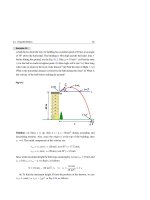
Example 21.9

A solid sphere of radius R has a uniform volume charge density ρ and carries a
total positive charge Q. Find and sketch the electric field at any distance r away
from the sphere’s center.


714

21 Gauss’s Law

Solution: We divide the solution to 0 ≤ r ≤ R and r ≥ R.
(1) For 0 ≤ r ≤ R
When dealing with a spherically symmetric charge distribution, we chose a spherical Gaussian surface of radius r < R concentric with the charged sphere as shown
in Fig. 21.15.
Fig. 21.15

ρ

R

dA
r

E

Gaussian
sphere

By symmetry, the magnitude of the electric field is constant everywhere on the
→
→
spherical Gaussian surface and normal to the surface at any point, i.e. E // dA .
Thus:
→

→

E • dA =

E dA = E

dA = E(4π r 2 )

It is important to notice that the volume, say V , of the Gaussian sphere encloses
a net charge qin = ρV ; that is:
qin = ρV = ρ( 43 π r 3 )
We can now use Gauss’s law to find electric field as follows:
E

=

→

→

E • dA =
E=

Then:

qin
◦

ρ
r
3 ◦

⇒

E(4π r 2 ) =

ρ( 43 π r 3 )
◦

(0 ≤ r ≤ R)

Using the definition ρ = Q/( 43 π R3 ) and k = 1/(4π ◦ ), we get:
E=

Q
4π

3
◦R

r=k

Q
r
R3

(0 ≤ r ≤ R)


21.3 Applications of Gauss’s Law

715

(2) For r ≥ R
Again, because the charge distribution is spherically symmetric, we can construct
a Gaussian sphere of radius r > R concentric with the charged sphere, as shown
in Fig. 21.16.
Fig. 21.16

Q

dA
R

Gaussian
sphere

→

E

r

→

Just as when r < R, E • dA = E(4π r 2 ), but qin = Q. Thus, we can use
Gauss’s law to find the electric field as follows:
E

i.e.:

=

→

→

E • dA =

E=

1
4π

qin

⇒

◦

Q
Q
=k 2
2
r
r
◦

E(4π r 2 ) =

Q
◦

(r ≥ R)

Notice that this is identical to the result obtained for a point charge. Therefore, we
conclude that the electric field outside any uniformly charged sphere is equivalent
to that of a point charge located at the center of the sphere. At r = R, the two cases
give identical results E = kQ/R2 . A plot of E versus r is shown in Fig. 21.17. This
figure shows the continuation of E and its maximum at r = R.
Fig. 21.17

ρ
R
E=k

E

Q
r2

Q
E=k 3r
R

0

R

r


716

21 Gauss’s Law

Example 21.10

A thin spherical shell of radius R has a total positive charge Q distributed uniformly
over its surface. Find the electric field inside and outside the shell.
Solution: By symmetry, if any field exists inside the shell, it must be radial. Let us
construct a spherical Gaussian surface of radius r < R concentric with the shell,
see the cross sectional view in Fig. 21.18.
Fig. 21.18

+
Q

+

R

Gaussian
sphere

+

Spherical +
shell

+

r
+

+
+

Based on Gauss’s law, the lack of charge inside the surface indicates that
→

→

E • dA = E(4π r 2 ) = 0, or E = 0. Accordingly, we conclude that there is no
electric field inside a uniformly charged spherical shell.
Outside the shell, we construct a spherical Gaussian surface of radius r > R
concentric with the charged shell as shown in Fig. 21.19.
Fig. 21.19

Q

+

+
r

+
Spherical
shell

Gaussian
sphere

+
R

+

+
→

+
+

→

Symmetry suggests that E = constant on that surface and E is parallel to dA ,
→

→

i.e. E • dA = E(4π r 2 ). Since the net charge qin inside the Gaussian surface is
equal to the total charge Q on the shell, the shell is equivalent to a point charge
located at the center. That is:
E=

1
4π

Q
Q
=k 2
2
r
r
◦

(r > R).


21.4 Conductors in Electrostatic Equilibrium

21.4

717

Conductors in Electrostatic Equilibrium

Conductors contain free electrons that can move freely. When there is no net motion
of electrons within the conductor, the conductor is in electrostatic equilibrium and
has the following four properties:

(1) The electric field inside the conductor is zero (see Example 21.3).
(2) The excess charge on an isolated conductor lies on its outer surface (see Example
21.3).
(3) The electric field just outside a charged conductor at any point is perpendicular to
its surface and has a magnitude E = σ/ ◦ , where σ is the surface charge density
at that point (see Example 21.4).
(4) The surface charge density is greatest at locations where the radius of curvature
of the surface is smallest (see Chap. 22).
We can elaborate more about the first property by considering the conducting
slab in electrostatic equilibrium on the left of Fig. 21.20, where the free electrons are
→

uniformly distributed throughout the slab, i.e. E int = 0. When we place the slab in an
→
external electric field E ext as in the right part of Fig. 21.20, the free electrons move
to the left. In time, more negative and positive charges accumulate on the left and
right surfaces, respectively. These two planes of charge create an increasing internal
→

→

→

electric field E int inside the conductor. After awhile, E int will compensate E ext ,
→
→
→
resulting in a zero net electric field inside the conductor, i.e. E net = E ext − E int = 0.
The time to reach this new electrostatic equilibrium is of the order 10−6 s.

Before E net = 0

After

→

Eext

+
+
- E net = 0 +
+
+
-

Eint

→

Fig. 21.20 An external electric field E ext creates an internal electric field E int in the conductor such
→

that the net electric field E net is zero

Example 21.11

A conducting sphere of radius R carries a net positive charge 2Q. A conducting
spherical shell of inner radius R1 (R1 > R) and outer radius R2 carries a net negative charge −Q. This shell is concentric with the conducting sphere. Find the