Hafez a radi, john o rasmussen auth principles of physics for scientists and engineers 2 30

21.5 Exercises

723

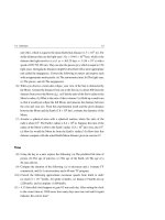
Fig. 21.28 See Exercise (8)

S2

r
q

S1
r
R

λ

Fig. 21.29 See Exercise (9)

S1
S4

q
−q
S3

S2

−2 q

2q

(10) A point charge q = 25 µC is located at the center of a sphere of radius
R = 25 cm. A circular cut of radius r = 5 cm is removed from the surface of the
sphere, see Fig. 21.30. (a) Find the electric flux that passes through that cut. (b)
Repeat when the cut has a radius r = 25 cm. Is the answer q/2 ◦ ?
Fig. 21.30 See Exercise (10)

r

q+
R

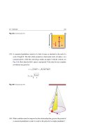
(11) A point charge q = 53.1 nC is located at the center of a cube of side a = 5 cm,
see Fig. 21.31. (a) Find the electric flux through each face of the cube. (b) Find
the flux through the four slanted surfaces of a pyramid formed from a vertex
on the center of the cube and one of its six square faces.


724

21 Gauss’s Law

Fig. 21.31 See Exercise (11)

y
a
q

+

x
a

z
a

(12) At an altitude h1 = 700 m above the ground, the electric field in a particular
region is E1 = 95 N/C downwards. At an altitude h2 = 800 m, the electric field
is E2 = 80 N/C downwards. Construct a Gaussian surface as a box of horizontal
area A and height lying between h1 and h2 , to find the average volume-charge
density in the layer of air between these two elevations.
(13) A point P is at a distance a = 10 cm from an infinite rod, charged with a uniform
charge per unit length λ = 5 nC/m. (a) Find the electric flux through a sphere
of radius r = 5 cm centered at P, see left of Fig. 21.32. (b) Find the electric flux
through a sphere of radius r = 15 cm centered at P, see right of Fig. 21.32.

r

-

+ +

P
r
a
λ
+ + + + +

P
a

-

+ +

+

+

+ +

λ
+

Fig. 21.32 See Exercise (13)

(14) A point charge q is located at a distance δ just above the center of the flat face
of a hemisphere of radius R as shown in Fig. 21.33. (a) When δ is very small,
use the argument of symmetry to find an approximate value for the electric flux
through the curved surface of the hemisphere. (b) When δ is very small,
use Gauss’s law to find an approximate value of the electric flux flat through
curved

the flat surface of the hemisphere.


21.5 Exercises

725

Fig. 21.33 See Exercise (14)

q

δ

R

Section 21.3 Applications of Gauss’s Law
(15) An infinite horizontal sheet of charge has a charge per unit area σ = 8.85 µC/m2 .
Find the electric field just above the sheet.
(16) A nonconductive wall carries a uniform charge density σ = 8.85 µC/cm2 . Find
the electric field 7 cm away from the wall. Does your result change as the
distance from the wall increases such that it is much less than the wall’s dimensions?
(17) Two infinitely long, nonconductive charged sheets are parallel to each other.
Each sheet has a fixed uniform charge. The surface charge density on the left
sheet is σ while on the right sheet is −σ, see Fig. 21.34. Use the superposition
principle to find the electric field: (a) to the left of the sheets, (b) between the
sheets, and (c) to the right of the sheets.
Fig. 21.34 See Exercise (17)

+
σ +
+
+
+
+
L

−σ

B

R

(18) Repeat the calculations for Exercise 17 when: (i) both the sheets have positive uniform surface charge densities σ, and (ii) both the sheets have negative
uniform surface charge densities −σ.
(19) A thin neutral conducting square plate of side a = 80 cm lies in the xy-plane,
see Fig. 21.35. A total charge q = 5 nC is placed on the plate. Assuming that


726

21 Gauss’s Law

the charge density is uniform, find: (a) the surface charge density on the plate,
(b) the electric field just above the plate, and (c) the electric field just below the
plate.
Fig. 21.35 See Exercise (19)

z
a
a

y
x

(20) A long filament has a charge per unit length λ = −80 µC/m. Find the electric
field at: (a) 10 cm, (b) 20 cm, and (c) 100 cm from the filament, where distances
are measured perpendicular to the length of the filament.
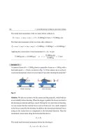
(21) A uniformly charged straight wire of length L = 1.5 m has a total charge

Q = 5 µC. A thin uncharged nonconductive cylinder of height = 2 cm and
radius r = 10 cm surrounds the wire at its central axis, see Fig. 21.36. Using
reasonable approximations, find: (a) the electric field at the surface of the cylinder and (b) the total electric flux through the cylinder.
Fig. 21.36 See Exercise (21)

Q

+
+
+
+ r
L
+
+
+

(22) A thin nonconductive cylindrical shell of radius R = 10 cm and length
L = 2.5 m has a uniform charge Q distributed on its curved surface, see
Fig. 21.37. The radial outward electric field has a magnitude 4 × 104 N/C at
a distance r = 20 cm from its axis (measured from the midpoint of the shell).


21.5 Exercises

727

Find: (a) the net charge on the shell, and (b) the electric field at a point r = 5 cm
from its axis.
Fig. 21.37 See Exercise (22)

R
Q
E

r

L

(23) A long non-conducting cylinder of radius R has a uniform charge distribution
of density ρ throughout its volume. Find the electric field at a distance r from
its axis where r < R?
(24) A thin spherical shell of radius R = 15 cm has a total positive charge Q = 30 µC
distributed uniformly over its surface, see Fig. 21.38. Find the electric field at:
(a) 10 cm and (b) 20 cm from the center of the charge distribution.
Fig. 21.38 See Exercise (24)

Q +

+
+

R

Spherical
shell
+

+
+

+
+

(25) Two concentric thin spherical shells have radii R1 = 5 cm and R2 = 10 cm. The
two shells have charges of the same magnitude Q = 3 µC, but different in sign,
see Fig. 21.39. Use the shown three Gaussian surfaces S1 , S2 , and S3 to find the
electric field in the three regions: (a) r < R1 , (b) R1 < r < R2 , and (c) r > R2 .
(26) A particle with a charge q = −60 nC is located at the center of a non-conducting
spherical shell of volume V = 3.19 × 10−2 m3 , see Fig. 21.40. The spherical
shell carries over its interior volume a uniform negative charge Q of volume
density ρ = −1.33 µC/m3 . A proton moves outside the spherical shell in a
circular orbit of radius r = 25 cm. Calculate the speed of the proton.


728

21 Gauss’s Law

Fig. 21.39 See Exercise (25)

S3

−Q

S2

Q

R2
R1

S1

Spherical
shells
Fig. 21.40 See Exercise (26)

Q
–

–
–

q

–
–

Spherical
shell

– –
–

–
– –

–

– –

–
–

–

–

r
–
– –

Point
charge

–
–

+e
+
– Proton

–

(27) A solid non-conducting sphere is 4 cm in radius and carries a 7.5 µC charge
that is uniformly distributed throughout its interior volume. Calculate the
charge enclosed by a spherical surface, concentric with the sphere, of radius
(a) r = 2 cm and (b) r = 8 cm.
(28) A solid non-conducting sphere of radius R = 20 cm has a total positive charge
Q = 30 µC that is uniformly distributed throughout its volume. Calculate the
magnitude of the electric field at: (a) 0 cm, (b) 10 cm, (c) 20 cm, (d) 30 cm,

and (e) 60 cm from the center of the sphere.
(29) If the electric field in air exceeds the threshold value Ethre = 3 × 106 N/C, sparks
will occur. What is the largest charge Q can a metal sphere of radius 0.5 cm
hold without sparks occurring?
(30) The charge density inside a non-conducting sphere of radius R varies as
ρ = α r (C/m3 ), where r is the radial distance from the center of the sphere.
Use Gauss’s law to find the electric field inside and outside the sphere.
(31) A solid sphere of radius R with a center at point C1 has a uniform volume
charge density ρ. A spherical cavity of radius R/2 with a center at point C2
is then scooped out and left empty, see Fig. 21.41. Point A is at the surface of
the big sphere and collinear with points C1 and C2 . What is the magnitude and
direction of the electric field at points C1 and A?


21.5 Exercises

729

Fig. 21.41 See Exercise (31)

A

C1

R

C2

R /2

Section 21.4 Conductors in Electrostatic Equilibrium
(32) A non-conducting sphere of radius R and charge +Q uniformly distributed
throughout its volume is concentric with a spherical conducting shell of inner
radius R1 and outer radius R2 . The shell has a net charge −Q, see Fig. 21.42.
Find an expression for the electric field as a function of the radius r when:
(a) r < R (within the sphere). (b) R < r < R1 (between the sphere and the
shell). (c) R1 < r < R2 (inside the shell). (d) r > R2 (outside the shell). (e) What
are the charges on inner and outer surfaces of the conducting shell?
Fig. 21.42 See Exercise (32)

−Q

Q

R

R1

R2

c

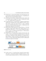
(33) A large, thin, copper plate of area A has a total charge Q uniformly distributed
over its surfaces. The same charge Q is uniformly distributed over the upper
surface of a glass plate, which is identical to the copper plate, see Fig. 21.43.
(a) Find the surface charge density on each face of the two plates. (b) Compare
the electric fields just above the center of the upper surface of each plate.


730

21 Gauss’s Law

Q

Copper plate

Q

Glass plate

Fig. 21.43 See Exercise (33)

(34) A thin, long, straight wire carries a charge per unit length λ. The wire lies
along the axis of a long conducting cylinder carrying a charge per unit length
3λ. The cylinder has an inner radius R1 and an outer radius R2 , see Fig. 21.44.
(a) Use a Gaussian surface inside the conducting cylinder to find the charge
per unit length on its inner and outer surfaces. (b) Use Gauss’s law to find the
electric field E outside the wire. (c) Sketch the electric field E as a function of
the distance r from the wire’s axis.
Fig. 21.44 See Exercise (34)

3λ

λ

R1

R2

(35) An uncharged solid conducting sphere of radius R contains two cavities.
A point charge q1 is placed within the first cavity, and a point charge q2 is
placed within the second one. Find the magnitude of the electric field for r > R,
where r is measured from the center of the sphere.


22

Electric Potential

Newton’s law of gravity and Coulomb’s law of electrostatics are mathematically
identical. Therefore, the general features of the gravitational force introduced in
Chap. 6 apply to electrostatic forces. In particular, electrostatic forces are conservative. Consequently, it is more convenient to assign an electric potential energy
U to describe any system of two or more charged particles. This idea allows us to
define a scalar quantity known as the electric potential. It turns out that this concept
is of great practical value when dealing with devices such as capacitors, resistors,
inductors, batteries, etc, and when dealing with the flow of currents in electric circuits.

22.1

Electric Potential Energy
→

The electric force that acts on a test charge q placed in an electric field E (created by
→
→
a source charge distribution) is defined by F = qE . For an infinitesimal displacement
d→
s 1 , the work done by the conservative electric field is:
→

→

dW = F • d →
s = qE • d →
s

(22.1)

According to Eq. 6.39, this amount of work corresponds to a change in the potential
energy of the charge-field system given by:
→

→

dU = −dW = −F • d →
s = −qE • d →
s

(22.2)

For a finite displacement of the charge from an initial point A to a final point B,
the change in electric potential energy U = UB − UA of the charge-field system
1

When dealing with electric and magnetic fields, it is common to use this notation to represent an
infinitesimal displacement vector that is tangent to a path through space.

H. A. Radi and J. O. Rasmussen, Principles of Physics,
Undergraduate Lecture Notes in Physics, DOI: 10.1007/978-3-642-23026-4_22,

© Springer-Verlag Berlin Heidelberg 2013

731


732

22 Electric Potential

is given by integrating along any path that the charge can take between these two
points. Thus:
B

U = UB − UA = −WAB = −q

→

E • d→
s

(22.3)

A

This integral does not depend on the path taken from A to B because the electric force
is conservative.
For convenience, we usually take the reference configuration of the charge-field
system when the charges are infinitely separated. Moreover, we usually set the corresponding reference potential energy to be zero. Therefore, we assume that the
charge-field system comes together from an initial infinite separation state at ∞ with
U∞ = 0 to a final state B with UB . We also let W∞B represent the work done by the

electrostatic force during the movement of the charge. Thus:
B

UB = −W∞B = −q

→

E • d→
s

(22.4)

∞

Although the electric potential energy at a particular point UB (or simply U) is
associated with the charge-field system, one can say that the charge in the electric
field has an electric potential energy at a particular point UB . You should always
keep in mind the fact that the electric potential energy is actually associated with the
→
charge plus the source charge distribution that establishes the electric field E.
Moreover, when defining the work done on a certain charged particle by the
electric field, you are actually defining the work done on that certain particle by the
→
electric force due to all the other charges that actually created the electric field E
in which that certain particle moved.
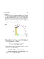
Example 22.1

In the air above a particular region near Earth’s surface, the electric field is
uniform, directed downwards, and has a value 100 N/C, see Fig. 22.1. Find the
change in the electric potential energy of an electron released at point A such that

the electrostatic force due to the electric field causes it to move up a distance
s = 50 m.
Solution: The change in the electric potential energy of the electron is related to
the work done on the electron by the electric field given by Eq. 22.3. Since the


22.1 Electric Potential Energy

733

electron’s displacement is upwards and the electric field is directed downwards,
i.e. θ = 180◦ , then we have:
B

U = −q

→

E • d→
s = −(−e)

A

B

E ds cos 180◦
A

B

= −eE

ds = −eE(sB − sA ) = −eEs
A

= −(1.6 × 10−19 C)(100 N/C)(50 m)
= −8 × 10−16 J

Fig. 22.1

-

s

F
e

B

-

A

E

Notice that the sign of the electron’s charge is used in this calculation. Thus, during
the 50 m ascent of the electron, the electric potential of the electron decreases by
8 × 10−16 J. Also, from Eq. 22.3, the work done by the electrostatic force on the
electron is:
WAB = − U = 8 × 10−16 J

22.2

Electric Potential

The electric potential energy depends on the charge q. However, the electric potential
energy per unit charge U/q has a unique value at any point and depends only on the
electric field (or alternatively on the source-charge distribution). This quantity is
called the electric potential V (or simply the potential). Thus:
V =

U
q

(22.5)


734

22 Electric Potential

This equation implies that the electric potential is a scalar quantity.
Spotlight
Electric potential is a scalar quantity that characterizes an electric field and is
independent of any charge that may be placed in the field.

The electric potential difference V (or simply the potential difference)
between two points A and B in an electric field is defined as the difference in the electric potential energy per unit charge between the two points. Thus, dividing Eq. 22.3
by q leads to:
V = VB − VA =

WAB
U
=−
=−
q
q

B

→

E • d→
s

(22.6)

A

It is clear that the electric potential difference between A and B depends only on
the source-charge distribution, and is equal to the negative of the work done by the
electrostatic force per unit charge. The SI unit of both the electric potential and
the electric potential difference is joule per coulomb, or volt (abbreviated by V).
That is:
1 V = 1 J/C

(22.7)

From this unit, we see that the joule is one coulomb times 1 V (J = CV). Additionally, the volt unit allows us to adopt a more convenient unit for the electric field.
From Eq. 22.6, the volt unit also has the units of electric field times distance. Then

we have:
1 N/C = 1 V/m

(22.8)

Spotlight
Electric field can be expressed as the rate of change of electric potential with
position.

From now on, we shall express values of electric fields in volts per meter (V/m)
rather than newtons per coulomb (N/C).


22.2 Electric Potential

735

Suppose we move a particle of an arbitrary charge q from point A to point B
by applying a force on it and changing its kinetic energy. The applied force must
perform work WAB (app), while the electric field does work WAB . From Eq. 6.54, the
change in the kinetic energy of the particle is:
K = WAB (app) + WAB

(22.9)

Now suppose the kinetic energy of the particle does not change during the move.
Then, Eq. 22.9 reduces to:
WAB (app) = −WAB

(22.10)

Since Eq. 22.6 gives q V = −WAB , then we have:
WAB (app) = q V

(22.11)

In atomic and nuclear physics, we use a convenient unit of energy called electronvolt (eV). One electron-volt (1 eV) is the energy equal to the work required to move
a single elementary charge e, such as that of an electron or a proton, through an
electric potential difference of exactly one volt (1 V). To find the value of this unit,
one can use Eq. 22.11 where q = 1.6 × 10−19 C and

V = 1 V, Thus:

1 eV = (1.6 × 10−19 C)(1 V) = (1.6 × 10−19 C)(1 J/C) = 1.6 × 10−19 J
(22.12)
An electron that strikes the screen of a typical TV set may have a speed of
4 × 107 m/s. This corresponds to a kinetic energy of 7.28 × 10−16 J, which is equivalent to 4.55 keV. In other words, such an electron has to be accelerated from rest
through a potential difference of 4.55 kV to reach a speed of 4 × 107 m/s.
Equations 22.3 and 22.6 hold true for both discrete and continuous source distributions, and for both uniform and varying fields. In the following sections, we
calculate the electric potential for various cases.

22.3

Electric Potential in a Uniform Electric Field

Displacement Parallel to a Field
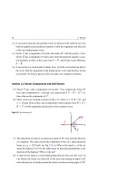
Let us calculate the potential difference between two points A and B separated by a
→
distance |→
s | = d, where →

s is a displacement along a uniform field E , see Fig. 22.2.
Then, Eq. 22.6 gives:


736

22 Electric Potential

Fig. 22.2 A uniform electric

A

field pointing downwards and
→

d→
s is along E. The electric

ds

d

potential at point B is lower
than that at point A

B
E
B

V = VB − VA = −

B

→

E • d→
s =−

A

B

(E cos 0◦ )ds = −E
A

ds

(22.13)

A

Integrating ds along a straight line gives (sB − sA ) = d. Thus:
V = VB − VA = −Ed

(Along the field)

(22.14)

The negative sign means that the electric potential at point B is lower than that at
point A, i.e. VB < VA . In fact, electric field lines always point in the direction of

decreasing electric potential.
If a charge q moves along the field from point A to point B, then according to
Eq. 22.6, the change in the electric potential energy U of the charge-field system
is given by U = q V. Then, substituting with Eq. 22.14, we get the following:
U = q V = −qEd

(Along the field)

(22.15)

(1) If q is positive (i.e. q = +|q|) and the charge moves in the direction of the field
from A to B, then U = −|q|Ed is negative. This means that the positive chargefield system loses electric potential energy. Also, since WAB = − U, this means
that the electric field does positive work WAB on the positive charge during this
motion. Furthermore, if this positive charge is released from rest at point A, it
accelerates downwards, gaining kinetic energy K = WAB when it reaches point
B. Thus:
K = − U = +|q|Ed

(Along the field for positive q)

(22.16)

(2) If q is negative (i.e. q = −|q|), and the charge moves in the direction of the field
from A to B, then U = +|q|Ed is positive. This means that the negative chargefield system gains electric potential energy. In order for the negative charge to
move along the field, an external agent must apply a force and do positive work
WAB (app) during that motion. For motion with zero acceleration from A to B,


22.3 Electric Potential in a Uniform Electric Field

737

this positive work compensates the negative work WAB done on the negative
charge by the field.
Similar steps can be performed when the displacement →
s is opposite to the field
from point A to point B, see Fig. 22.3, which leads to:
V = VB − VA = Ed

(Opposite the field)

(22.17)

Fig. 22.3 Same as Fig. 22.2
except that d →
s is opposite

B

→

to E

d

ds
A
E

If a charge q moves against the field from A to B, then according to Eq. 22.6, the

change in the electric potential energy U of the charge-field system is given by
U = q V. By substitution with Eq. 22.17 we get the following:
U = q V = qEd

(Opposite the field)

(22.18)

(1) If q is positive (i.e. q = +|q|), and the charge moves against the field from A to B,
then U = +|q|Ed is positive. This means that the positive charge-field system
gains electric potential energy. In order for the positive charge to move against
the field, an external agent must apply a force and do positive work WAB (app)
during that motion. For motion with zero acceleration from A to B, this positive
work compensates for the negative work WAB done on the positive charge by the
electric field.
(2) If q is negative (i.e. q = −|q|) and is released from rest at A, it will accelerate
upwards to B. In this case V = VB −VA = +Ed, and U = −|q| V = −|q|Ed
(loss of electric potential energy). Since WAB = − U, then WAB = +|q|Ed, i.e.
the electric field does positive work on the negative charge during its motion
from A to B. The gain in kinetic energy
K = − U = +|q|Ed

K = WAB is thus:

(Opposite the field for negative q)

This gain is the same as for a positive charge moving along the field.

(22.19)

738

22 Electric Potential

Arbitrary Displacement in the Field
Now, let us calculate the potential difference between two points A and B when the
→

displacement →
s has an arbitrary direction with respect to the uniform field E , see
Fig. 22.4a. Equation 22.6 gives:
B

V = VB − VA = −

→

→

E • d→
s = −E •

A

B

d→
s

(22.20)

A

Path of constant
potential

A
s

Equipotential
surfaces

d

B

C
E

V1
V2
V3

E

(a)

(b)

Fig. 22.4 (a) When the uniform electric field lines point down, the electric potential at point B is lower
than that at point A. Points B and C are at the same electric potential. (b) Portions of equipotential surfaces
→

that are perpendicular to the electric field E

Integrating d →
s along the path gives →
sB − →
sA = →
s . Thus:
→

V = VB − VA = −E • →
s

(22.21)

When a charge q moves from A to B, the change in the electric potential energy U
of the charge-field system is given according to Eq. 22.6 by U = q V. Then, using
Eq. 22.21 we get:
→

U = q V = −qE • →
s

(From A to B)

(22.22)

→

From Fig. 22.4a, we notice that E • →
s = Es cos θ = Ed. Thus, any point in a plane
perpendicular to a uniform electric field has the same electric potential. We can see
this in Fig. 22.4a, where the potential difference VB − VA is equal to the potential
difference VC − VA ; that is VC = VB . All points that have the same electric potential
form what is called an equipotential surface, see Fig. 22.4b.


22.3 Electric Potential in a Uniform Electric Field

739

Example 22.2

The electric potential difference between two opposing parallel plates is 12 V,
while the separation between the plates is d = 0.4 cm. Find the magnitude of the
electric field between the plates.
Solution: We use Eq. 22.14, namely

V = VB −VA = −Ed, to find the magnitude

of the uniform electric field as follows:
E=

12 V
|VB − VA |
=
= 3,000 V/m (or N/C)

d
0.4 × 10−2 m

Example 22.3

Figure 22.5 shows two oppositely charged parallel plates that are separated by
a distance d = 5 cm. The electric field between the plates is uniform and has a
magnitude E = 10 kV/m. A proton is released from rest at the positive plate, see
Fig. 22.5. (a) Find the potential difference between the two plates. (b) Find the
change in potential energy of the proton just before striking the opposite plate.
(c) Calculate the speed of the proton when it strikes the plate.
Fig. 22.5

+ + + +

Proton

E
A

0

+

+

A

B

B

d
Solution: (a) Since the potential must be lower in the direction of the field, then
VA > VB in Fig. 22.5. According to Eq. 22.14 the potential difference between the
two plates along the field is:
V = VB − VA = −Ed = −(10 × 103 V/m)(5 × 10−2 m) = −500 V
(b) Equation 22.15 gives the change in potential energy as:
U = q V = e V = (1.6 × 10−19 C)(−500 V) = −8 × 10−17 J
The negative sign indicates that the potential energy of the proton decreases as
the proton moves in the direction of the field.


740

22 Electric Potential

(c) Using Eq. 22.16, we can find for the proton that:
K =− U
2
1
2 mp vB

vB =

−2 U
=
mp

−0=− U

−2(−8 × 10−17 J)
= 3.1 × 105 m/s
1.67 × 10−27 kg

Example 22.4

Redo Example 22.3, but this time with an electron that is released from rest at the
negative plate, see Fig. 22.6.
Fig. 22.6

+

E

+ + +

B

A

-

Electron

0

-

A

B
d

Solution: (a) Since the potential must be lower in the direction of the field,
then VB > VA in Fig. 22.6. Then, according to Eq. 22.17 the potential difference
between the two plates is:
V = VB − VA = +Ed = +(10 × 103 V/m)(5 × 10−2 m) = +500 V
This means that VB = VA + 500 V as expected, since point B lies on the positive
plate.
(b) From Eq. 22.18, we find for the electron that:
U = q V = −e V = −(1.6 × 10−19 C)(500 V) = −8 × 10−17 J
The negative sign indicates that the potential energy of the electron decreases as
the electron moves in the opposite direction of the field.
(c) From Eq. 22.19, we find for the electron that:
K =− U


22.3 Electric Potential in a Uniform Electric Field
2
1
2 me vB

vB =

−2 U
=
me

741

−0=− U

−2(−8 × 10−17 J)
= 1.33 × 107 m/s
9.11 × 10−31 kg

Although we are using the same constants of Example 22.3, with the same change
in potential energy of the electron as for the proton, the speed of the electron is
much greater than the speed of the proton because the electron’s mass is much
smaller.

22.4

Electric Potential Due to a Point Charge

To find the electric potential at a point located at a distance r from an isolated positive
point charge q, we begin with the general expression for potential difference:
B

VB − VA = −

→

E • d→
s

(22.23)

A

where A and B are two points having position vectors →
r A and →
r B , respectively, see
Fig. 22.7. In this representation, the origin is at q. According to Eq. 20.4, the electric
→
field at a distance r from the point charge is E = kq →
rˆ /r 2 = Er →
rˆ , where →
rˆ is a unit
→

vector directed from the charge to point P. The quantity E • d →
s , can be written as:
→
q ˆ →
E • d→
s = Er →
rˆ • d →
s =k 2 →
r • ds
r

(22.24)

Fig. 22.7 The potential
difference between points A

ds
E

and B due to a point charge q

rB

depends only on the radial
coordinates rA and rB

B

dr

r
+ q
A

rA

→
From Fig. 22.7, we see that →
rˆ • d →
s = 1 × ds × cos θ = dr. Then, E • d →
s =
Er dr, and Eq. 22.23 can be written as:


742

22 Electric Potential
rB

VB − VA = −

rB

Er dr = −kq
rA

Therefore:

r −2 dr = −kq −r −1

rA

VB − VA = kq

rB
rA

1
1
−
rB
rA

(22.25)

This result does not depend on the path between A and B, but depends only on the
initial and final radial coordinates rA and rB .
It is common to choose a reference point where VA = 0 at rA = ∞. With this

reference choice, the electric potential at any arbitrary distance r from a point charge
q will be given by:
V =k

q
r

(22.26)

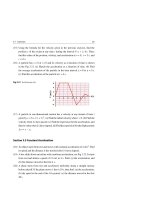
The sign of V depends on q. If r → 0, then V → +∞ or V → −∞ depending on
q. Figure 22.8 shows a plot for V in the xy-plane.
Fig. 22.8 A computer-

V

generated plot for the electric
potential V(r) of a single
point-charge in the xy-plane.
The predicted infinite value of
V(r) is not plotted

y
x
When many point charges are involved, we can get the resulting electric potential
at point P from the superposition principle. That is:
V =k

n

qn

,
rn

(n = 1, 2, 3, . . .)

(22.27)

where rn is the distance from the point P to the charge qn .

Electric Potential Energy of a System of Point Charges
The electric potential energy of a system of two point charges q1 and q2 can be
obtained first by having both charges placed at rest and set infinitely apart. Then, by