Hafez a radi, john o rasmussen auth principles of physics for scientists and engineers 2 31

22.4 Electric Potential Due to a Point Charge

743

bringing q1 by itself from infinity and putting it in place as shown in Fig. 22.9a, we
do no work for such a move. The electric potential at point P which is at a distance
r12 from q1 is given by Eq. 22.26 as VP = kq1 /r12 . Later, by bringing q2 without
acceleration from infinity to point P at a distance r12 from q1 , as shown in Fig. 22.9b,
we must do work W∞P (app) for such a move, since q1 exerts an electrostatic force
on q2 during the move.

P

VP

k

r12

q1
r12

q2
r12
U

k

q1

q1

(a)

q 1 q2
r12

(b)

Fig. 22.9 (a) The potential VP at a distance r12 from a point charge q1 . (b) The potential energy of two
point charges is U = kq1 q2 /r12

We can calculate W∞P (app) by using

K = W∞P (app) + W∞P = 0, i.e.

W∞P (app) = −W∞P . When we replace q2 by the general charge q in Eq. 22.6, we
find that:
VP − V∞ =

UP − U∞
W∞P
=−
q2
q2

(22.28)

Setting V∞ as well as U∞ to zero (our reference point at ∞), we get:
VP =

UP

W∞P (app)
=
q2
q2

⇒

UP = W∞P (app) = q2 VP

(22.29)

Substituting with VP = kq1 /r12 , we can generalize the electric potential energy of a
system of two point charges q1 and q2 separated by a distance r12 as follows:
U=k

q1 q2
r12

(22.30)

If the charges have the same sign, we have to do positive work to overcome their
mutual repulsion, and then U is positive. If the charges have opposite signs, we have


744

22 Electric Potential

to do negative work against their mutual attraction to keep them stationary, and then
U is negative.

When the system consists of more than two charges, we calculate the potential
energy of each pair and add them algebraically. For instance, the total potential energy
of three charges q1 , q2 , and q3 is:
q1 q2
q1 q3
q2 q3
+
+
r12
r13
r23

U=k

(22.31)

Example 22.5

Two charges q1 = 2 µC and q2 = − 4 µC are fixed in their positions and separated
by a distance d = 10 cm; see Fig. 22.10a. (a) Find the total electric potential at the
point P in Fig. 22.10a. (b) Find the change in potential energy of the two charges
when a third charge q3 = 6 µC is brought from ∞ to P, see Fig. 22.10b. (c) What
is the total electric potential energy of the three charges?

P

+

d
q1 +

d

d

d

d
-

q2

q1 +

(a)

q3

d

-

q2

(b)

Fig. 22.10

Solution: (a) For two charges, Eq. 22.27 gives:
VP = k

2 × 10−6 C −4 × 10−6 C
q2
q1
+
= (9 × 109 N.m2 /C2 )
+
d
d
0.1 m
0.1 m

= −1.8 × 105 V
(b) When we replace q3 by the charge q of Eq. 22.6, and bring q3 from infinity
to point P, this equation gives:
U = q3 (VP − V∞ ) = (6 × 10−6 C)(−1.8 × 105 V − 0) = −1.08 J


22.4 Electric Potential Due to a Point Charge

745

(c) The total electric potential energy of the three charges is:
q1 q3
q2 q3
q1 q2
+
+
d
d

d
[(2)(−4)
+ (2)(6) + (−4)(6)] × 10−12 C2
= (9 × 109 N.m2 /C2 )
= −1.8 J
0.1 m

U=k

22.5

Electric Potential Due to a Dipole

As introduced in Chap. 20, an electric dipole consists of a positive charge q+ = +q
and an equal-but-opposite negative charge q− = −q separated by a distance 2a. Let
us find the electric potential at a point P in the xy-plane as shown in Fig. 22.11a. We
assume that V+ is the electric potential produced at P by the positive charge, and that
V− is the electric potential produced at P by the negative charge.
y

y
P(x,y)
r

r

r

r

q

-

( a,0)

r

r
r

y

q
+
O
(a,0)
xa
x a

q

x

q
-

+

O

x

2a
(b)

(a)

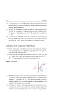
Fig. 22.11 (a) The electric potential V at point P(x, y) due to an electric dipole located along the x-axis
with a length 2a. Point P is at a distance r from the midpoint O of the dipole, where OP makes an angle θ
with the dipole’s x-axis. (b) When P is very far, the lines of length r+ and r− are approximately parallel
to the line OP

The total electric potential at P is thus:
V = V+ + V− = k

q+
q−
1
1
+k
= kq
−
r+
r−
r+
r−

= kq

r− − r+
r+ r−

(22.32)

2 = (x − a)2 + y2 and r 2 = (x + a)2 +
From the geometry of Fig. 4.11a, we find that r+
−
y2 . Accordingly, Eq. 22.32 becomes:

V = kq

1
(x

− a)2

+ y2

−

1
(x + a)2 + y2

(22.33)


746

22 Electric Potential

Note that V = ∞ at P(x = a, y = 0) and V = −∞ at P(x = −a, y = 0). Figure 22.12
shows a plot of the general shape of V in the xy-plane.
Fig. 22.12 A computer-

V
y

generated plot of the electric
potential V in the xy-plane for
an electric dipole. The
predicted infinite values of V
are not plotted

x

Because naturally occurring dipoles have very small lengths, such as those possessed by many molecules, we are usually interested only in points far away from
the dipole, i.e. r

2a. Considering these conditions, we find from Fig. 22.11b that:
r− − r+

2a cos θ,

and

r− r+

r2

(22.34)

When substituting these approximate quantities in Eq. 22.32, we find that:
V = kq

2a cos θ
r2

(r

2a)

(22.35)

As introduced in Chap. 20, the product of the positive charge q and the length of
the dipole 2a is called the magnitude of the electric dipole moment, p = 2aq. The
direction of →
p is taken to be from the negative charge to the positive charge of the
→
→
dipole, i.e. p = p i . This indicates that the angle θ is measured from the direction

of →
p . Using this definition, we have:
V =k

p cos θ
r2

(r

2a)

(22.36)

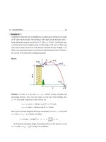
Example 22.6

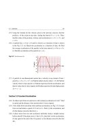
Find the electric potential along the axis of the electric dipole at the four points
A, B, C, and D in Fig. 22.13.


22.5 Electric Potential Due to a Dipole

747

y
D

-q

C

-

B

+q

A

+

x

O
(-a,0)

(a,0)

Fig. 22.13

Solution: We use Eq. 22.32 with r+ and r− as the distance from each point to the
positive and negative charges, respectively:
(1) For point A in Fig. 22.13, we have x > a. Therefore, r+ = x − a and r− =
a + x. The electric potential VA is:
1
1
1
1
−
= kq
−
r+
r−
x−a a+x
2k qa
(x
a)
x2

VA = kq

=

2k qa
x 2 − a2

(VA positive)

(2) For point B in Fig. 22.13, we have 0 < x < a. Therefore r+ = a − x and
r− = a + x. The electric potential VB is:
VB = kq

1
1
−
r+
r−

= kq

1
1
−
a−x a+x

=

2kq
x

a2 − x 2

(VB positive)

(3) For point C in Fig. 22.13, we have −a < x < 0. Therefore r+ = a − x and
r− = a + x. The electric potential VC is:
VC = kq

1
1
−
r+
r−

= kq

1
1
−
a−x a+x

=

2kq
x
a2 − x 2

(VC negative)

(4) For point D in Fig. 22.13, we have x < −a. Therefore r+ = a − x and

r− = −x − a. The electric potential VD is:
1
1
−
r+
r−
2kqa
− 2
(x
x

VD = kq

22.6

= kq

1
1
+
a−x a+x

=−

2kqa
− a2

x2

−a)

(VD negative)

Electric Dipole in an External Electric Field

Consider an electric dipole of electric dipole moment →
p is placed in a uniform
→
external electric field E , as shown in Fig. 22.14. Do not get confused between the


748

22 Electric Potential

field produced by the dipole and this external field. In addition, we assume that the
→

vector →
p makes an angle θ with the external field E .

+q +

2a

p
o

−F

θ

F
E

p

⊗

θ

E

- -q

(b)

(a)

Fig. 22.14 (a) An electric dipole has an electric dipole moment →
p in an external uniform electric

→
→
field E . The angle between →
p and E is θ. The line connecting the two charges represents their rigid

connection and their center of mass is assumed to be midway between them. (b) Representing the electric

→

dipole by a vector →
p in the external electric field E and showing the direction of the torque →
τ into the

page by the symbol ⊗

→

→

Figure 22.14 shows a force F , of magnitude qE in the direction of E , is exerted on
→
the positive charge, and a force −F , of the same magnitude but in opposite direction,
is exerted on the negative charge. The resultant force on the dipole is zero, but since
the two forces do not have the same line of action, they establish a clockwise torque
τ→ about the center of mass of the two charges at o. The magnitude of this torque
about o is:
τ = (2a sin θ )F

(22.37)

Using F = qE and p = 2aq, we can write this torque as:
τ = (2aq sin θ )E = pE sin θ

(22.38)

The vector torque τ→ on the dipole is therefore the cross product of the vectors →
p
→
and E . Thus:

→

τ→ = →
p ×E

(22.39)

The effect of this torque is to rotate the dipole until the dipole moment →
p is aligned
→
with the electric field E .


22.6 Electric Dipole in an External Electric Field

749

Potential energy can be associated with the orientation of an electric dipole in an
electric field. The dipole has the least potential energy when it is in the equilibrium
→
orientation, which occurs when →
p is along E . On the other hand, the dipole has the
→

greatest potential energy when →
p is antiparallel to E . We chose the zero-potential→
energy configuration when the angle between →
p and E is 90◦ .
According to Eq. 22.3, U = UB − UA = −WAB , we can find the electric

potential energy of the dipole by calculating the work done by the field from the
initial orientation θ = 90◦ , where UA ≡ U(90◦ ) = 0, to any orientation θ, where
UB ≡ U(θ ). In addition, we use the relation W = τ dθ, to find U(θ ) as follows:
U(θ ) − U(90◦ ) = −W90◦ →θ = −

θ

τ dθ

(22.40)

90◦

Letting U(θ ) ≡ U, U(90◦ ) = 0, τ = pE sin θ, and integrating we get:
U = −pE cos θ

(22.41)

This relation can be written in vector form as follows:
→

U = −→
p •E

(22.42)

Equation 22.42 shows the least and greatest value of U as follows:
180°
p

τ max
p

90°

τ

E
p

22.7

E

E

Electric Potential Due to a Charged Rod

For a Point on the Extension of the Rod
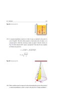
Figure 22.15 shows a rod of length L with a uniform positive charge density λ and a
total charge Q. In this figure, the rod lies along the x-axis and point P is taken to be
at the origin of this axis, located at a distance a from the left end. When we consider
a segment dx on the rod, the charge on this segment will be dq = λ dx.


750

22 Electric Potential

y

P

dx

x

+ + + + + + + + + + + +
dq
L

0
a

x

Fig. 22.15 The electric potential V at point P due to a uniformly charged rod lying along the x-axis. The
electric potential due to a segment of charge dq at a distance x from P is k dq/x. The total electric potential
is the algebraic sum of all the segments of the rod

The electric potential dV at P due to this segment is given by:
dV = k

dq
λ dx
=k
x
x

(22.43)

We obtain the total electric potential at P due to all the segments of the rod by
integrating from one end of the rod (x = a) to the other (x = a + L) as follows:
a+L

V =

dV =

k
a

λ dx
= kλ
x

a+L

x −1 dx = kλ| ln x|a+L
= kλ {ln(a + L) − ln a}
a
a

Therefore:
V = kλ ln

a+L
a

=

kQ
a+L
ln
L
a

(22.44)

For a Point on the Perpendicular Bisector of the Rod
A rod of length L has a uniform positive charge density λ and a total charge Q. The
rod is placed along the x-axis as shown in Fig. 22.16. Assuming that P is a point on
the perpendicular bisector of the rod and is located a distance a from the origin of
the x-axis, then the charge of a segment dx on the rod will be dq = λ dx.
The electric potential dV at P due to this segment is:
dV = k

λ dx
dq
=k
r
r

(22.45)

The total electric potential at P due to all segments of the rod is given by two times
the integral of dV from the middle of the rod (x = 0) to one of its ends (x = L/2).
Thus:


22.7 Electric Potential Due to a Charged Rod

751

Fig. 22.16 A rod of length L

y

with a uniform positive charge

P

density λ and an electric
potential dV at point P due to

a

a charge segment

r
dq

+ + + + + + + + + ++ +
x
0
dx
L

x=L/2

V =2

L/2

dV = 2kλ
x=0

0

dx
r

x

(22.46)

To perform the integration of this expression, we relate the variables x and r. From
√
the geometry of Fig. 22.16, we use the fact that r = x 2 + a2 . Therefore, Eq. 22.46
becomes:
L/2

V = 2kλ
0

dx
(x 2 + a2 )1/2

(22.47)

From the table of integrals in Appendix B, we find that:

(x 2

dx
= ln(x +
+ a2 )1/2

V = 2kλ ln(x +

x 2 + a2 )

Thus:
= 2kλ ln(L/2 +

Therefore:

V = 2kλ ln

x 2 + a2 )

(22.48)

L/2
0

(L/2)2 + a2 ) − ln(a)

L/2 +

(L/2)2 + a2
a

(22.49)

When we use the fact that the total charge Q = λL, we get:
V =

L/2 +
2kQ
ln
L

(L/2)2 + a2
a

(22.50)


752

22 Electric Potential

For a Point Above One End of the Rod
When a point P is located at a distance a from one of the rod’s ends, see Fig. 22.17,
we can perform similar calculations to find that:
L+
kQ
ln
V =
L

√
L 2 + a2
a

Fig. 22.17 A setup similar to

y

Fig. 22.16 except P is above

P

one end

a

0

22.8

(22.51)

r
dq

++++ +++++ +++
x
dx
L

x

Electric Potential Due to a Uniformly Charged Arc

Assume that a rod has a uniformly distributed total positive charge Q. Assume now
that the rod is bent into an arc of radius R and central angle φ rad, see Fig. 22.18a.
To find the electric potential at the center P of this arc, we first let λ represent the
linear charge density of this arc, which has a length Rφ. Thus:
λ=

Q
Rφ

(22.52)

For an arc element ds subtending an angle dθ at P, we have:
ds = R dθ

(22.53)

Therefore, the charge dq on this arc element will be given by:
dq = λ ds = λ R dθ

(22.54)

To find the electric field at P, we first calculate the differential electric potential
dV at P due to the element ds of charge dq, see Fig. 22.18b, as follows:
dV = k

dq

= kλ dθ
R

(22.55)


22.8 Electric Potential Due to a Uniformly Charged Arc

753

P

P

R

R

R
Q

+

+

θ

Q

+

+ +
+
+ + + +

+

+

(a)

R

dθ
dq

++
+
+ + + + ++
s
ds
(b)

+

Fig. 22.18 (a) A circular arc of radius R, central angle φ, and center P has a uniformly distributed
positive charge Q. (b) The figure shows how to calculate the electric potential dV at P due to an arc
element ds having a charge dq

The total electric potential at P due to all elements of the arc is thus:
φ

V =

dV = kλ

dθ = kλφ
0

Using Eq. 22.52, we get:
V = kλφ = k

Q
R

(22.56)

This expression is identical to the formula of a point charge. The reason for this is
that the distance between P and each charge element on the arc does not change and
its orientation is irrelevant.

22.9

Electric Potential Due to a Uniformly Charged Ring

Assume that a ring of radius R has a uniformly distributed total positive charge Q,
see Fig. 22.19. Additionally, assume that a point P lies at a distance a from the center
of the ring along its central perpendicular axis, as shown in the same figure.
To find the electric potential at P, we first calculate the electric potential dV at P
due to a segment of charge dq as follows:
dV = k

where r =

√

dq
r

R2 + a2 is a constant distance for all elements on the ring.

(22.57)


754

22 Electric Potential

Fig. 22.19 A ring of radius R

z

having a uniformly distributed

P

positive charge Q. The figure

Q

shows how to calculate the

a

r

electric potential dV at an
axial point P due to a segment

R

of charge dq on the ring

dq

Thus, the total electric potential at P is:
V =

k
k dq
=√
√
2
2
2
R +a
R + a2

dV =

dq

(22.58)

Since dq represents the total charge Q over the entire ring, then the total electric
potential at P will be given by:
kQ
V =√
R2 + a2

(22.59)

22.10 Electric Potential Due to a Uniformly Charged Disk
Assume that a disk of radius R has a uniform positive surface charge density σ, and
a point P lies at a distance a from the disk along its central perpendicular axis, see
Fig. 22.20.
Fig. 22.20 A disk of radius R

z

has a uniform positive surface
charge density σ. The ring

P

Ring

a

Charge per
unit area

shown has a radius r and a

Disk

radial width dr

dr
r

R

To find the electric potential at P, we divide the disk into concentric rings, then
calculate the electric potential at P for each ring by using Eq. 22.59, and summing
up the contribution of all the rings.


22.10 Electric Potential Due to a Uniformly Charged Disk

755

Figure 22.20 shows one such ring, with radius r, radial width dr, and surface area
dA = 2π rdr. Since σ is the charge per unit area, then the charge dq on this ring is:
dq = σ dA = 2π rσ dr

(22.60)

Using this relation in Eq. 22.59, and replacing V with dV, R with r, and Q with
dq = 2π rσ dr, we can calculate the electric potential resulting from this ring as
follows:
k

2rdr
dV = √
(2π rσ dr) = π kσ √
2
2
r +a
r 2 + a2

(22.61)

To find the total electric potential, we integrate this expression with respect to the
variable r from r = 0 to r = R. This gives:
R

V =

(r 2 + a2 )−1/2 (2r dr)

dV = π kσ

(22.62)

0

To solve this integral, we transform it to the form un du = un+1 /(n + 1) by setting
u = r 2 + a2 , and du = 2r dr. Thus, Eq. 22.62 becomes:
u=R2 +a2

R

V = π kσ

2 −1/2

(r + a )
2

(2r dr) = π kσ

0

= π kσ

u−1/2 du

u=a2

u=R2 +a2
u1/2

1/2

u=a2

= π kσ

(R2

+ a2 )1/2
1/2

(22.63)
−

a
1/2

Rearranging the terms, we find that:
V = 2π kσ

√
R2 + a2 − a

(22.64)

Using k = 1/4π ◦ , where ◦ is the permittivity of free space, it is sometimes preferable to write this relation as:
V =

σ √ 2
R + a2 − a
2 ◦

(22.65)


756

22 Electric Potential

22.11 Electric Potential Due to a Uniformly Charged Sphere

A solid sphere of radius R has a uniform volume charge density ρ and carries a total
positive charge Q. First, we find the electric potential in the region r ≥ R by using
the electric field obtained in Example 21.9. In this region, we found that E is radial
and has a magnitude:
Er = k

Q
r2

(r ≥ R)

(22.66)

This is the same as the electric field due to a point charge, and hence the electric
potential at any point of radius r in this region is given by:
Vr = k

Q
r

(r ≥ R)

(22.67)

The potential at a point on the surface of the sphere (r = R) is:
VR = k

Q
R

(22.68)

In the region 0 ≤ r ≤ R inside the sphere, we use the result of the electric field obtained
→

in Example 21.9. In this region, we found that E is radial and has a magnitude:
Er = k

Q
r
R3

(0 ≤ r ≤ R)

(22.69)

For a point that has a radius r in the region 0 ≤ r ≤ R, we can find the potential
difference between this point and any point on the surface with a radius R by using

→

E • d→
s = Er dr in Eq. 22.6. Thus:
r

Vr − VR = −

→

E • d→

s =−

R

r

Er dr = −k
R

Q r2
= −k 3
R 2

r=r
r=R

Q
R3

r

r dr
R

(22.70)

Q
= k 3 (R2 − r 2 )
2R

Using VR = kQ/R in the last result we reach to the following relation:
Vr = k

r2
Q
3− 2
2R
R

(0 ≤ r ≤ R)

(22.71)

At r = 0, we have V0 = 3kQ/2R, and at r = R, we get VR = kQ/R as expected.
Figure 22.21 sketches the electric potential in the two regions 0 ≤ r ≤ R and r ≥ R.


22.12 Electric Potential Due to a Charged Conductor

757

Fig. 22.21 A sketch of the

R

electric potential V (r) as a

r

function of r in the two regions

0 ≤ r ≤ R and r ≥ R. The curve
for the region 0 ≤ r ≤ R is

V0 =

parabolic and joins smoothly
with the curve for the region

r2
R2
Q
Vr = k r
Q

V

3k Q
2R

Vr = k 2R 3 −

2V
3 0

r ≥ R, which is hyperbola

0

r

R

22.12 Electric Potential Due to a Charged Conductor
Assume that a solid conducting sphere of radius R carries a net positive charge Q
as shown in Fig. 22.22a. We found in Chap. 21 that the charge on this equilibrium
conductor must reside on its outer surface. Furthermore, the electric field inside the
conductor is zero and the electric field just outside its surface is perpendicular to the
surface.

E
Charged
conductor

Q
VR = k
R

A
B
+
+
+
R
+
+
+ + +
V

0
(a)

Charged conductor

Uniform
surface
charge
density
Vr = k

R

r

Q
r

+
++
+
+
+
+

+

++

E
+
+

++
++
+ ++

Nonuniform surface
charge density
(b)

Fig. 22.22 (a) A sketch of the electric potential V (r) as a function of r in the two regions 0 ≤ r ≤ R
and r ≥ R for a charged spherical conductor. When r = R, the formulas in the regions match. (b) For a
nonsymmetrical conductor, the surface charge density is greatest at the points where the radius of curvature
of the surface is least

Consider two arbitrary points A and B on the surface of this spherical conductor,
→

see Fig. 22.22a. Since E ⊥ d →
s along the path AB on the surface of that conductor,
→
then E • d →
=
0.
Using
this
result
along with Eq. 22.6, we find that:
s

758

22 Electric Potential
B

VB − VA = −

→

E • d→
s =0

(22.72)

A

During equilibrium, the electric potential V is constant everywhere on the surface of
this charged spherical conductor and equal to VR = kQ/R, or VR = 4π kRσ in terms
of the surface charge density σ.
Furthermore, because the electric field is zero inside the conductor, the electric
potential would be constant everywhere inside the conductor and is equal to its value
at the surface.
Outside this spherical conductor, the electric potential is Vr = kQ/r for r ≥ R.
Figure 22.22a plots V against r and shows the dependence of V (r) on r for the whole
range of r.
If the conductor is not symmetric as in Fig. 22.22b, the electric potential is constant everywhere on its surface, but the surface charge density is not uniform. Since
V = const. and V ∝ Rσ, i.e. Rσ = const., the surface charge density increases as
the radius of curvature decreases.

22.13 Potential Gradient

We defined the potential difference between two points A and B as the negative of
→
the work done by the electric field E per unit charge in moving the charge from A
to B, see Eq. 22.6. Thus:
B

VB − VA = −

→

E • d→
s

(22.73)

A

If we write VB − VA =

B
A

dV = −

B→
A

E • d→
s , then we must have:
→

dV = −E • d →
s

(22.74)
→

If the electric field has only one component Ex along the x-axis, then E • d →
s = Ex dx.
The last equation becomes dV = −Ex d x, or:
Ex = −

dV
dx

(22.75)


22.13 Potential Gradient

759

Thus, the x component of the electric field is equal to the negative of the derivative
of the electric potential with respect to x.
→
If the field is radial, i.e. V = V (r) as introduced in Sect. 22.4, then E • d →
s = Er dr
and we can express Eq. 22.74 as:
Er = −
→

→

→

dV
dr

→

(22.76)
→

→

→

Generally, E = Ex i + Ey j + Ez k and d →
s = dx i + dy j + dz k . Then:
→

dV = −E • d →
s = −Ex dx − Ey dy − Ez dz

(22.77)

When V = V (x, y, z), the chain rule of differentiation gives:
dV =

∂V

∂V
∂V
dx +
dy +
dz
∂x
∂y
∂z

(22.78)

By comparing the last two equations, we get the potential gradients:
Ex = −

∂V
∂x

Ey = −

∂V
∂y

Ez = −

∂V
∂z

(22.79)

Example 22.7

From the formulas of the electric potential given by Eqs. 22.26, 22.44, 22.59, and
22.65, find the formulas of the electric fields.
Solution: To get the electric field from the electric potential, we use Eqs. 22.76
or 22.79 depending on the system coordinates.
(1) From the point-charge formula given by Eq. 22.26, we have a radial electric
field. Thus:
Er = −

d
q
dr −1
q
dV
=−
k
= −kq
=k 2
dr
dr
r
dr
r

(Identical to Eq. 20.4)

(2) From the charged-rod formula given by Eq. 22.44, our variable is the distance a from the end of the rod. Thus:
d
a+L
d

dV
=−
kλ ln
= −kλ {ln(a + L) − ln a}
da
da
a
da
1
kλL
1
−
=
(Identical to Eq. 20.26)
= −kλ
a+L a
a(a + L)

Ea = −


760

22 Electric Potential

(3) From the charged-ring formula given by Eq. 22.59, our variable is the
distance a from the center of the ring. Thus:
dV
d
=−

da
da
kQa
= 2
(R + a2 )3/2

Ea = −

kQ
√
R2 + a2

= −kQ(− 21 )(R2 + a2 )−3/2 (2a)

(Identical to Eq. 20.50)

(4) From the charged-disk formula given by Eq. 22.65, our variable is the
distance a from the center of the disk. Thus:
d
σ
dV
=−
da
da 2 ◦
a
σ
1− √
=
2
2 ◦

R + a2

Ea = −

R2 + a2 − a

=−

σ
2 ◦

1
2

(R2 + a2 )−1/2 (2a) − 1

(Identical to Eq. 20.56)

The expressions that we have arrived at for the electric potentials established by
simple charge distributions are presented in Table 22.1.
Table 22.1 Electric potential due to simple charge distributions
Charge distribution
Two oppositely charged conducting
plates separated by a distance d

Electric potential
V = VB − VA = − Ed Along the field
V = VB − VA = Ed Opposite the field
q
r

Single point charge q

V =k

Charged ring of radius R with a uniformly distributed total charge Q

kQ
V=√
R2 + a2

Disk of radius R having a uniform
surface charge density σ

V=

Charge q uniformly distributed on
the surface of a conducting sphere
of radius R

V =

r >0

a≥0

σ √ 2
R + a2 − a
2 ◦
⎧ q

⎪
k
⎪
⎨ r

r ≥R

⎪
⎪
⎩k q
R

r ≤R

a>0


22.14 The Electrostatic Precipitator

761

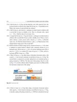
22.14 The Electrostatic Precipitator
Electrostatic precipitators are highly efficient filtration devices used to remove particles from a flowing gas (such as air). They do this using the force of an induced
electrostatic charge. Such devices remove particulate matter from combustion gases,
and as a result reduce air pollution. Most precipitators on the market today are capable
of eliminating more than 99% of the ash from smoke.
A schematic diagram of an electrostatic precipitator is shown in Fig. 22.23.
Applied between the central wire and the duct walls, where smoke is flowing up
the duct, is a large voltage of several thousand volts (50–100 kV). To generate an
electric field that is directed toward the wire, the wire is maintained at a negative

electric potential with respect to the walls. Such a large electric field produces a
discharge around the wire, which causes the air near the wire to contain electrons,
positive ions, and negative ions such as O−
2.

Insulator

Without Precipitator

Cleaned air

Polluted air

weight
Dirt

Dirt out
Fig. 22.23 (a) A schematic diagram of an electrostatic precipitator. The high negative electric potential
on the central wire creates a discharge in the vicinity of the wire, causing dirt to fall down. (b) Pollution
from a power-plant’s chimney not equipped with an electrostatic precipitator

Polluted air enters the duct from the bottom and moves near the coiled wire. The
discharge creates electrons and negative ions, which accelerate toward the outer wall
due to the force of the electric field. Consequently, the dirt particles become charged
by collisions and ion capture. Because most of the charged dirt particles are negative,


762

22 Electric Potential

they are drawn to the walls by the electric field. Periodic shaking of the duct loosens
the particles, which are then collected at the bottom.

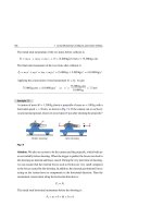
22.15 The Van de Graaff Generator
When a charged conductor is connected to the inside of a hollow conductor, all the
charge is transferred to the outer surface of the hollow conductor regardless of any
charge already retained by the conductor. The generator invented by Robert Van de
Graaff makes use of this principle, where a “conveyor belt” carries out the charge
continuously, see the schematic diagram of Fig. 22.24a.

A

F

B
E

D

C

/>
(a)

(b)

Fig. 22.24 (a) The charge in the Van de Graaff generator is deposited at E and transferred to the dome
at F. (b) By touching the dome, each hair strand becomes charged and repels strands around it

This generator consists of a hollow metallic dome A supported by an insulating
stand B mounted on a grounded metal base C and a non-conducting belt D running
over two non-conducting pulleys. The belt is charged as a result of the discharge
produced by the metallic needle at E, which is maintained at a positive electric
potential of about 104 V. The positive charge on the moving belt is transferred to the
dome by the needle at F, regardless of the dome’s electric potential. It is possible to
increase the potential of the dome until electrical ionization occurs in the air. Since the
ionization breakdown of air occurs at an electric field of about 3 × 106 V/m, a sphere
of 1 m can be raised to maximum of Vmax = ER = (3 × 106 V/m)(1 m) = 3 × 106 V.
The dome’s electric potential can be increased further by placing the dome in vacuum
and by increasing the radius of the sphere.


22.16 Exercises

763

22.16 Exercises
Section 22.1 Electric Potential Energy
(1) A charge q = 2.5 × 10−8 C is placed in an upwardly uniform electric field of
magnitude E = 5 × 104 N/C. What is the change in the electric potential energy
of the charge-field system when the charge is moved (a) 50 cm to the right? (b)
80 cm downwards? (c) 250 cm upwards at an angle 30◦ from the horizontal?
(2) Redo question 1 to calculate the work done on the charge q by the electric field.
(3) Redo question 1 to calculate the work done on the charge q by an external agent
such that the charge moves in each case without changing its kinetic energy.

Section 22.2 Electric Potential
(4) How much work is done by an external agent in moving a charge q =
−9.63 × 104 C from a point A where the electric potential is 10 V to a point

B where the electric potential is −4 V? How many electrons are there in this
charge? Is this number related to any of the known physical constants?

Section 22.3 Electric Potential in a uniform Electric Field
(5) The electric potential difference between the accelerating plates in the electron
gun of a TV tube is 5,550 V, while the separation between the plates is d = 1.5 cm.
Find the magnitude of the uniform electric field between the plates.
(6) An electron moves a distance d = 2 cm when released from rest in a uniform
electric field of magnitude E = 6 × 104 N/C. (a) What is the electric potential
difference through which the electron has passed? (b) Find the electron’s speed
after it has moved that distance?
(7) Two large parallel metal plates are oppositely charged with a surface charge
density of magnitude σ = 1.2 nC/m2 , see Fig. 22.25. (a) Find the electric field
between the plates. (b) If the electric potential difference between these two
plates is 10 V, what is the distance between the plates?
(8) A uniform electric field of magnitude 3 × 102 N/C is directed in the positive x
direction as shown in Fig. 22.26. In this figure, the coordinates of point A are
(0.3, −0.2) m and the coordinates of point B are (−0.5, 0.4) m. Calculate the
potential difference VB − VA using: (a) the path A → C → B. (b) the direct path
A → B.


764

22 Electric Potential

Fig. 22.25 See Exercise (7)

+

+σ

−σ

+
E
+
+

Fig. 22.26 See Exercise (8)

y
E
B

C
x
A

(9) An insulated rod has a charge Q = 20 µC and a mass m = 0.05 kg. The rod is
released from rest at a location A in a uniform electric field of magnitude 104 N/C
directed perpendicular to the field, see Fig. 22.27 and neglect gravity. (a) Find
the speed of the rod when it reaches location B after it has traveled a distance
d = 0.5 m. (b) Does the answer to part (a) change when the rod is released at an
angle θ = 45◦ relative to the electric field?
Fig. 22.27 See Exercise (9)

B

A

A= 0

m

E
+ + + + + +

Q

+ + + + + +

Q

B

m
d

Section 22.4 Electric Potential Due to a Point Charge
(10) (a) What is the electric potential at a distances 1 and 2 cm, from a proton? (b)
What is the potential difference between these two points?


22.16 Exercises

765

(11) Redo Exercise 10 for an electron.
(12) At a distance r from a particular point charge q, the electric field is 40 N/C and

the electric potential is 36 V. Determine: (a) the distance r, (b) the magnitude
of the point charge q.
(13) Two point charges q1 = +2 µC and q2 = −6 µC are separated by a distance
L = 12 cm, see Fig. 22.28. Find the point at which the resultant electric potential
is zero.
Fig. 22.28 See Exercise (13)

q1

q2
L

+

-

(14) Two charges q1 = −2 µC and q2 = +2 µC are fixed in their positions and separated by a distance d = 10 cm, see the top part of Fig. 22.29. (a) What is the
electric field at the origin due these two charges? (b) What is the electric potential at the origin and the electric potential energy of the two charges? (c) Find
the change in potential energy of the two charges when a third charge q3 = 2 µC
is brought from ∞ to O, see the bottom part of Fig. 22.29.
Fig. 22.29 See Exercise (14)

q2

q1
-

+

x

O
d
q1

q3

q2

-

+
O
d

+

x

(15) Three equal charges q1 = q2 = q3 = 6 nC are located at the vertices of an equilateral triangle of side a = 6 cm, see Fig. 22.30. Find the electric potential at
point P, which is at the center of the base of the triangle.
Fig. 22.30 See Exercise (15)

+ q3
a
q1 +

a
P
a

+

q2


766

22 Electric Potential

(16) Three negative point charges are placed at the vertices of an isosceles tri√
angle as shown in Fig. 22.31. Given that a = 2 cm, q1 = q3 = −2 nC, and
q2 = −4 nC, find the electric potential at point P (which is midway between q1
and q3 ).
Fig. 22.31 See Exercise (16)

q1

P

a

q2

-

- q3

a

Section 22.5 Electric Potential Due to a Dipole
(17) An electric dipole is located along the x-axis with its center at the origin. The
dipole has a negative charge −q at (−a, 0) and a positive charge +q at (+a, 0),
see Fig. 22.11. Show that the electric potential on the y-axis is zero for any value
of y.
(18) Assume that a third positive charge +q is placed at the origin of the dipole of
Fig. 22.11, so that the new configuration will be as show in Fig. 22.32. Show
that the electric potential for far away points (such as P) on the dipole axis is
given by:
V (x) =

kq
2a
1+
x
x

−q

+q

+q

-

+

+

-a

0

+a

a)

P

x
Fig. 22.32 See Exercise (18)

(x

x


22.16 Exercises

767

(19) The permanent electric dipole moment of the ammonia molecule NH3 is
p = 4.9 × 10−30 C.m. Find the electric potential due to an ammonia molecule
at a distance 52 nm away along the axis of the dipole.

Section 22.6 Electric Potential Due to a Charged Rod
(20) A non-conductive rod has a uniform positive charge density +λ, a total charge
Q along its right half, a uniform negative charge density −λ, and a total charge
−Q along its left half, see Fig. 22.33. (a) What is the electric potential at point
A? (b) What is the electric potential at point B?

Fig. 22.33 See Exercise (20)

y

B
-Q

+Q

y

A
x

+ + + + + +
0

L /2

2L

Section 22.7 Electric Potential Due to a Uniformly Charged Arc
(21) A non-conductive rod has a uniformly distributed charge per unit length −λ.
The rod is bent into a circular arc of radius R and central angle 120◦ , see
Fig. 22.34. Find the electric potential at the center of the arc.
Fig. 22.34 See Exercise (21)

P

R

R

120°
−λ

(22) A non-conductive rod has a uniformly distributed charge per unit length λ. Part
of the rod is bent into a semicircular arc of radius R and the rest is left as two
straight rod segments each of length R as shown in Fig. 22.35. Find the electric
potential at point P.