Hafez a radi, john o rasmussen auth principles of physics for scientists and engineers 2 32

Capacitors and Capacitance

23

In this chapter we introduce capacitors, which are one of the simplest circuit elements.
Capacitors are charge-storing devices that can store energy in the form of an electric
potential energy, and are commonly used in a variety of electric circuits.
Apart from being energy-storing devices, capacitors can be used to accumulate
charges relatively slowly during the charging process, or to minimize voltage variations in electronic power supplies, or to detect electromagnetic waves, such as when
tuning a radio receiver.
We shall first study the properties of capacitors and dielectrics, and follow that
by studying capacitors in combination, and finally studying capacitors as electric
charge-storing devices.

23.1

Capacitor and Capacitance

We can use a device called capacitor to store energy in the form of an electric
potential. Beyond serving as storehouses for electric potential energy, capacitors
have many uses in our electronic and microelectronic age.
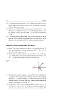
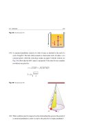
Figure 23.1a shows the basic elements of an air-filled capacitor. It consists of
two isolated conductors of any arbitrary shape, each of which carries an equal but
opposite charge of magnitude Q.
Figure 23.1b shows a more convenient and practical arrangement of an air-filled
capacitor, called a parallel-plate capacitor, consisting of two parallel conducting
plates of area A separated by a distance d of air. We represent a capacitor of any
geometry by the symbol (
capacitor.

), which is based on the structure of a parallel plate

H. A. Radi and J. O. Rasmussen, Principles of Physics,
Undergraduate Lecture Notes in Physics, DOI: 10.1007/978-3-642-23026-4_23,
© Springer-Verlag Berlin Heidelberg 2013

773


774

23 Capacitors and Capacitance

−Q

+Q

−Q

+Q

Area A

E

E

d

(a)

(b)

Fig. 23.1 (a) A capacitor made up of two conductors carrying an equal but opposite charge of magnitude
Q. (b) A parallel-plate capacitor made up of two plates of area A separated by a distance d. Each plate
carries an equal but opposite charge of magnitude Q

Experiments show that the magnitude of the charge on a capacitor is directly
proportional to the potential difference between its conductors; i.e. Q ∝ V ; which
can be written as Q = C

V. Thus:
C=

Q
V

(23.1)

The proportionality constant C is called the capacitance of the capacitor and depends
on the shape and separation of the conductors. Furthermore, the charge Q and the
potential difference V are always expressed in Eq. 23.1 as positive quantities to
produce a positive ratio C = Q/ V. Hence:
Spotlight
The capacitance C of a capacitor is defined as the ratio of the magnitude of
the charge on either conductor to the magnitude of the potential difference
between the conductors.
The SI unit of the capacitance is coulomb per volt, or farad (abbreviated by F).
That is:
1 F = 1 C/V

(23.2)

The farad is a very large unit of capacitance. In practice, typical devices have capacitances ranging from microfarads (1 µF = 10−6 F), nanofarads (1 n F = 10−9 F), to
picofarads (1 p F = 10−12 F).


23.2

23.2

Calculating Capacitance

775

Calculating Capacitance

For a capacitor with a charge of magnitude Q, we can calculate the potential
difference V using the technique described in the preceding chapter. Then we
can use the expression C = Q/ V to calculate the capacitance for the capacitor
under consideration.

A Parallel-Plate Capacitor
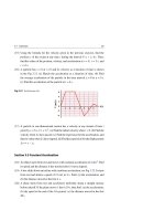
Figure 23.2a shows an uncharged parallel-plate capacitor of equal area A separated
by a distance d. The capacitor is connected in a circuit containing a battery B that
has a potential difference V and an open switch S. When the switch is closed,
the battery establishes an electric field in the wires and consequently charges flow
in the circuit to charge the capacitor with a charge of magnitude Q, see Fig. 23.2b.
Therefore, some of the stored chemical energy in the battery is transformed to the
→

capacitor in the form of an electric field E. Figure 23.2c shows the circuit schematic
to represent the battery, the symbol
to
diagram, where we use the symbol
represent the capacitor C, and the symbol
open switch is represented by the symbol

to represent the closed switch S. An
.
+Q

A

E

−Q

C

A
S

S
ΔV

S

d

d

B

ΔV

B

B

ΔV

(a)

(b)

(c)

Fig. 23.2 (a) A parallel-plate capacitor is connected to a battery B and an open switch S. (b) When S
is closed, each capacitor plate will carry equal but opposite charges of magnitude Q. (c) A schematic
diagram of the circuit with symbols representing the elements used

To find the relation between the capacitance and the geometry of this parallel-plate
capacitor, we first note that the magnitude of the surface charge density on either


776

23 Capacitors and Capacitance

plate is σ = Q/A. Then according to Example 21.6, the magnitude of the electric

field between the plates (assuming it uniform) is:
E=

σ

Since the positive potential difference

◦

=

Q
◦A

(23.3)

V across the battery and the plates are

identical, then according to Eq. 22.17 we have:
V = Ed =

Qd
◦A

(23.4)

Substituting this result into Eq. 23.1, we get:
C=

Q

Q
=
V
Qd/ ◦ A

Thus, the capacitance of the parallel-plate capacitor is:
C=

◦A

d

(Parallel-plate capacitor)

(23.5)

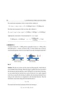
A Cylindrical Capacitor
Figure 23.3a shows a cylindrical capacitor of length composed of a solid cylindrical
conductor of radius a having a charge Q and a coaxial cylindrical conducting shell
of radius b having a charge −Q. Thus, the magnitude of the linear charge density on
either the cylinders is λ = Q/ . We assume that
b and hence neglect the fringing
(non-uniformity) of the electric field at the cylinders’ ends.
Figure 23.3b shows a cross-sectional view of the cylindrical capacitor. The electric
field in the region between the cylinders is radial and perpendicular to the axis of
the cylinders. In Chap. 21, we showed using Gauss’s law that the electric field of
a cylindrical charge distribution having a linear charge density λ is radial and is
given by:
Er = 2k

λ
r

(k = 1/4π ◦ )

The same formula applies here since the charge on the outer shell does not contribute
to any cylindrical Gaussian surface having a < r < b.


23.2

Calculating Capacitance

−Q

Q

a

b

777
Coaxial cable

Cross sectional view

Copper wire
Insulator

Cylindrical

conducting
shell
Gaussian
cylinder

b

r
E

Q

Copper
mesh
Outside
insulator

a

Path of
integration

−Q

Solid
cylindrical
conductor

(b)

(a)

Fig. 23.3 (a) A cylindrical capacitor in the form of a cylindrical solid conductor surrounded by a coaxial
shell. (b) A cross-sectional view of the capacitor showing a Gaussian cylinder of radius a < r < b

The potential difference Vb − Va between the cylinders is given by:
b

Vb − Va = −

b

→

E •d →
s =−

a

b

Er d r = −2 k λ
a

a

b
dr
= −2 kλ ln
r

a

(23.6)

Therefore, the magnitude of the potential difference between the cylinders is
V = |Vb − Va | = 2kλ ln (b/a). Substituting this result into Eq. 23.1 and using the
fact that λ = Q/ , we get:
C=

Q
Q
=
V
2k(Q/ ) ln (b/a)

Thus, the capacitance of a cylindrical capacitor of length is:
C=

2k ln (b/a)

= 2π

◦

ln (b/a)

(Cylindrical capacitor)

(23.7)

In addition, the capacitance per unit length of this configuration is:
C

=

1
= 2π
2k ln (b/a)

◦

1
ln (b/a)

(Cylindrical capacitor)

(23.8)

A Spherical Capacitor
Figure 23.4a shows a three-dimensional spherical capacitor consisting of a solid
spherical conductor of radius a having a charge Q and a concentric spherical shell
of radius b having a charge −Q.


778

23 Capacitors and Capacitance

Cross sectional view
−Q

b
Q

a

Spherical
conducting
shell
Solid
spherical
conductor

Spherical
conducting
shell
Gaussian
sphere

b

r
E

Q

a

Solid
spherical

conductor

Path of
integration − Q

(a)

(b)

Fig. 23.4 (a) A spherical capacitor consists of a spherical solid conductor surrounded by a concentric
spherical shell. (b) A cross-sectional view across the center of the spheres showing a Gaussian sphere of
radius a < r < b

Figure 23.4b shows a cross-sectional view of the spherical capacitor. As shown
in Chap. 21, the electric field outside a spherically symmetric charge distribution is
radial and is given by:
Er = k

Q
r2

This result applies only to the field between the spheres since the charge on the
outer spherical shell does not contribute to any spherical Gaussian surface having
a < r < b, see Fig. 23.4b.
The potential difference Vb − Va between the spheres is given by:
b

→

E •d →

s =−

Vb − Va = −
a

b

b

Er dr = −k Q
a

1
= kQ
r

b

= kQ
a

a

dr
r2

(23.9)

1 1
−

b a

Therefore, the magnitude of the potential difference between the spheres is
|Vb − Va | = kQ (b − a)/ab. Substituting this result into Eq. 23.1, we obtain:
C=

V=

Q
Q
=
V
kQ (b − a)/ab

Thus, the capacitance of the spherical capacitor is:
C=

ab
= 4π
k (b − a)

◦

ab
(b − a)

(Spherical capacitor)

(23.10)

23.2

Calculating Capacitance

779

An Isolated Sphere
The capacitance of a single isolated spherical conductor of radius R can be obtained
by assuming that the missing second conducting sphere has an infinite radius.
The electric field lines that leave or enter the isolated spherical conductor must
therefore end at infinity. For practical purposes, the walls of the room in which the
spherical conductor is housed can serve as our missing sphere of infinite radius. This
proves that any single conductor has a capacitance.
To find the capacitance of the isolated spherical conductor, we rearrange Eq. 23.10
to be as follows:
C=

a
k (1 − a/b)

Then we let b → ∞ and replace a by R in this formula to find the following relation:

C=

R
= 4π
k

◦R

(Isolated sphere)

(23.11)

Note that all the formulas derived so far for the capacitance [Eqs. 23.5, 23.7, 23.10,
and 23.11] involve the constants 1/k or ◦ multiplied by a quantity that has the
dimension of a length. Thus, the units of k and
respectively.

◦

may be expressed as m/F and F/m,

Example 23.1

The plates of a parallel-plate capacitor are separated in air by a distance d = 1 mm.
(a) Find the capacitance of this capacitor if its area is A = 1 cm2 . (b) What must
be the plate area if its capacitance is to be 1 F?
Solution: (a) From Eq. 23.5, we have:
C=

◦A

d

=

(8.85 × 10−12 F/m)(1 × 10−4 m2 )
= 8.85 × 10−13 F = 0.885 pF

(1 × 10−3 m)

(b) From Eq. 23.5, we have:
A=

Cd
◦

=

(1 F)(1 × 10−3 m)
= 1.13 × 108 m2
(8.85 × 10−12 F/m)

This is an area of a square that has a side of more than 10.6 km. Therefore,
the farad is indeed a large unit. However, modern technology has permitted the


780

23 Capacitors and Capacitance

construction of a 1 F capacitor of a very modest size. This capacitor is used as a
backup power supply (up to many months) for computer memory chips in case
of a power failure.

Example 23.2

Show that the capacitance of the cylindrical capacitor shown in Fig. 23.3a
approaches the capacitance of a parallel-plate capacitor if the separation d between

the two cylinders is very small.
Solution: When d = b − a is very small, then d/a must also be very small. If we
use the approximation ln (1 + x) ≈ x for x 1, in the natural logarithm of the
denominator of Eq. 23.7, we find that:
ln

b
a

= ln

a+d
a

= ln 1 +

d
a

≈

d
(When d/a
a

1)

Then, using the surface area of the inner cylinder A = 2π a , we find that Eq. 23.7
approaches Eq. 23.5 as follows:
C = 2π

Example 23.3

◦

ln (b/a)

≈ 2π

◦

d/a

=

◦

2π a
◦A
=
d
d

(Spherical Capacitor)

(a) How much charge is stored in a spherical capacitor consisting of two concentric spheres of radii a = 20 cm and b = 21 cm if the potential difference between
them is 200 V? (b) Show that if the separation d between the two spheres is small
compared to their radii, then the capacitance is given by the parallel-plate capacitance formula ◦ A/d. (c) Does the answer to part (b) apply to part (a)? (d) Find
the capacitance of the inner sphere of part (a) if it is isolated.
Solution: (a) For concentric spheres, Eq. 23.10 is used to calculate the capacitance

as follows:
C=

(0.2 m)(0.21 m)
ab
=
= 4.67×10−10 F = 0.467 nF
k (b − a) (9 × 109 m/F)(0.21 m − 0.2 m)

Then, by using Eq. 23.1, the magnitude of the charge on each sphere will be:
Q = C V = (4.67 × 10−10 F)(200 V) = 93.4 nC


23.2 Calculating Capacitance

781

(b) When the separation d = b − a is small, we can write the surface area of
each sphere as A ≈ 4π a2 ≈ 4π b2 ≈ 4π ab. Then, we have:
C = 4π

◦

ab
=
(b − a)

◦

4π ab

◦A
≈
d
d

(c) Since the separation d in part (a) is very small compared to the radii of the
spheres, then according to part (b) the capacitance is:
C≈

◦A

d

=

4π a2
d

◦

=

4π(0.2 m)2 (8.85 × 10−12 F/m)
= 4.45×10−10 F
(1 × 10−2 m)

This is very close to the answer 4.67 × 10−10 F obtained in part (a).
(d) Substituting with R = a = 20 cm in Eq. 23.11, we find that:
C = 4π

23.3

◦R

= 4π(8.85 × 10−12 F/m)(0.2 m) = 2.22 × 10−11 F

Capacitors with Dielectrics

An Electrical Description of Dielectrics
Capacitance was found to increase when a non-conducting material (such as oil,
rubber, plastic, glass, or waxed paper) is inserted between the capacitor’s plates. These
non-conducting materials are called dielectrics. If the dielectric completely fills the
space between the plates, the capacitance is found to increase by a dimensionless
factor κ (the Greek alphabet Kappa), called the dielectric constant.

Fixed Charge
Consider a parallel-plate capacitor without a dielectric to have a capacitance C◦ , a
charge Q◦ , and potential difference V◦ , i.e. C◦ = Q◦ / V◦ , see Fig. 23.5a. When
a dielectric is inserted between the plates, see Fig. 23.5b, the potential difference
between the plates is found to decrease to a value V related to V◦ by the relation:
V =
Note that, κ > 1 because

V < V◦ .

V◦
κ

(23.12)

23 Capacitors and Capacitance

C°

Fig. 23.5 (a) A capacitor

+ Q°

with capacitance C◦ has a

− Q°

C

+ Q°

− Q°

Dielectric

782

charge Q◦ when the potential
difference between the plates is
V◦ . (b) When the capacitor’s
charge is maintained, inserting
a dielectric reduces the
potential difference to
where

0

0

V,

V < V◦

Voltmeter

Voltmeter

Δ V°
(a)

ΔV
(b)

After inserting the dielectric, the capacitance C of the capacitor can be obtained
from Eq. 23.1 as follows:
C=

Q◦
Q◦
=κ
V◦ /κ
V◦

Q◦

=
V

(23.13)

Using C◦ = Q◦ / V◦ , we find that:
C = κ C◦

(23.14)

This indicates that the capacitance increases by a factor κ when the dielectric completely fills the space between the plates of the capacitor. Using Eq. 23.5, C◦ = ◦ A/d,
the capacitance becomes:
C=

κ

◦A

d

=

A
d

(23.15)

where = κ ◦ and is known as the permittivity of the dielectric.
→
On the other hand, if E ◦ is the electric field without the dielectric, then a reduction

of the potential difference from V◦ to V = V◦ /κ means that the electric field
→
→
→
decreases from E ◦ to E = E ◦ /κ. That is:
→

→

E◦
E =
κ

(23.16)


23.3 Capacitors with Dielectrics

783

Fixed Potential Difference
Now, consider a parallel-plate capacitor without a dielectric, having a capacitance
C◦ , a charge Q◦ , and connected to a battery that has a potential difference V◦ , i.e.
C◦ = Q◦ / V◦ , see Fig. 23.6a. If the dielectric is inserted between the plates while
the potential difference is held constant by keeping the capacitor connected to the
battery, see Fig. 23.6b, then the capacitance has to increase as before by the relation
C = κC◦ . Consequently, the magnitude of the charge on the capacitor has to increase
by a factor κ according to the relation:
Q = κQ◦

(23.17)

The extra charge comes from the battery attached to the capacitor.

+ Q°

C°

Δ V°

− Q°

B

(a)

+Q

C

Dielectric

−Q

Δ V°

B

(b)

Fig. 23.6 (a) A capacitor with capacitance C◦ has a charge Q◦ when connected to a battery that has
a potential difference

V◦ . (b) When the potential difference is maintained by the battery, inserting a

dielectric increases the charge to Q, where Q = κQ◦

An Atomic Description of Dielectrics
The molecules of some dielectrics have randomly oriented permanent electric dipole
→
moments as shown in Fig. 23.7a. The presence of an external electric field E ◦ in such
materials (called polar dielectrics), will exert a torque on the dipoles, causing them
to partially align with the field, as shown in Fig. 23.7b. We can now describe the


784

23 Capacitors and Capacitance

dielectric as being polarized, and the degree of alignment depends generally on the
→

strength of E◦ .
+σ
Dielectric

-

+

- +

- +

- +

- +

- +

- +

- + - +

- +

- +

+σ

°

+

+

-

−σ

°

Dielectric

E

E°

Ei

E°

- +

(b)

-

+

(a)

+σ i

−σ i

-

- +

+

-

-

+

- +
-

+

+

-

°

Dielectric

+

+

- +

-

−σ

°

(c)

Fig. 23.7 (a) A dielectric that has randomly oriented molecules. (b) The partial alignment of molecules
→

in the presence of an external electric field E ◦ due to a charged parallel plate capacitor with a surface
charge density of magnitude σ◦ . (c) The formation of an induced charge density +σi and −σi on either
→

→

sides of the capacitor sets up an induced electric field E i . The resultant electric field E inside the dielectric
→

has the same direction as E ◦ but is less in magnitude

→
E◦

Even when the dielectric material is non-polar, the applied external electric field

tends to separate the centers of the positive and negative charges of the molecules,
producing induced electric dipole moments. Therefore, the induced electric dipole
moments tend to align with the external electric field, and the dielectric is polarized.
The net effect on the dielectric is the formation of an induced positive and negative
charge density +σi and −σi on the right and left faces of the dielectric, respectively,
→

see Fig. 23.7c. Therefore, an induced electric field Ei will be established in a direction
→
→
opposite to the external electric field E◦ . Accordingly, the net electric field E in the
dielectric will have a magnitude given by:
E = E◦ − Ei

(23.18)

In the case of the parallel-plate capacitor shown in Fig. 23.7c, we use the relations
E◦ = σ◦ / ◦ , Ei = σi / ◦ , and E = E◦ /κ = σ◦ / , to get:
σ◦
σi
σ◦
=
−
κ ◦
◦
◦

(23.19)

or
σi =

κ −1
σ◦
κ

(Parallel-plate capacitor)

(23.20)


23.3 Capacitors with Dielectrics

785

where σi < σ◦ because κ > 1. When the dielectric is replaced by a conductor, for
which E = 0, then Ei = E◦ and hence σi = σ◦ . This means that the induced charge
on the conductor is equal in magnitude but opposite in sign to that on the plates of
the parallel-plate capacitor.
Equation 23.15 indicates that the capacitance C increases drastically when d
diminishes. However, d is limited by the electric discharge that could occur through
the dielectric medium. Every dielectric material has a specific dielectric strength
Emax , which is the maximum value of the electric field that the dielectric can withstand without electrical breakdown. Above this value the dielectric breaks down
and forms a conducting path between the capacitor’s plates. The largest potential
difference Vmax that can be applied to a dielectric without exceeding the dielectric
strength is called the breakdown potential difference. In fact, insulating materials
have κ > 1 and their Emax is greater than that of air.
Table 23.1 displays approximate dielectric constants κ and dielectric strengths
Emax of some materials at room temperature.
Table 23.1 Approximate values of the dielectric constants and dielectric strengths of some materials at
room temperature

κ

Emax (106 V/m ≡ kV/mm)

Vacuum

1.00000

–

Air (1 atm)

1.00059

3

Teflon

2.1

60

Silicon oil

2.5

15

Mylar

3.2

7

Nylon

3.4

14

Paraffin-impregnated paper

3.5

11

Paper

3.7

16

Pyrex glass

5.6

14

Distilled Water

80

–

Material

Types of Capacitors
Low-voltage capacitors are usually made of metallic foil interlaced with thin sheets
of a dielectric material, made of either paraffin-impregnated paper or Mylar. The
metallic foil and dielectric are rolled into a cylinder to form a small package, see
Fig. 23.8a.


786

23 Capacitors and Capacitance

Paper

Metallic foil

Electrolyte

Plates
Oil

Contacts

Case

Metalllic foil + oxide layer

(a)

(b)

(c)

(d)

Fig. 23.8 (a) A low-voltage capacitor whose plates are separated by paper as a dielectric. (b) A highvoltage capacitor consisting of a number of plates separated by insulating oil as a dielectric. (c) An
electrolytic capacitor used to store a large amount of charge. (d) A variable air capacitor

High-voltage capacitors are usually made of a number of interwoven metallic
plates immersed in silicon oil, see Fig. 23.8b.
Large-charge storage capacitors consist of a metallic foil in contact with an electrolyte. When a voltage is applied between the foil and the electrolyte, a very thin
layer of metal oxide is formed on the foil, and that layer serves as a dielectric, see
Fig. 23.8c. Because the dielectric layer is very thin, the capacitance obtained with
this type is very large. Such capacitors are assigned a polarity, which is indicated by
positive and negative signs. If the polarity of the applied voltage is reversed, the oxide
layer is removed, and the capacitor starts conducting electricity instead of storing
charge.
Variable capacitors whose capacitance may vary are widely used in tuning circuits
of radio receivers. They are constructed from a set of fixed parallel-plates connected
together to form one plate of the capacitor, while the second set of movable plates
are connected together to form the other plate. The plates are separated by air as a
dielectric, see Fig. 23.8d.
Example 23.4

The parallel plates in Fig. 23.9a have an area A = 0.2 m2 and separation distance
d = 0.01 m. The original potential difference between them is V◦ = 300 V which
decreases to V = 100 V when a dielectric sheet fills the space between the plates,
see Fig. 23.9b. (a) Calculate the capacitance C◦ , the magnitude of the charge Q◦ ,
and the magnitude of the electric field E◦ . (b) Calculate the final capacitance C and

the dielectric constant κ. (c) Find the magnitudes of the induced charge density
σi , the induced electric field Ei , and the final electric field E.


23.3 Capacitors with Dielectrics

+σ

C°

°

+ Q°

−σ

E°

787

+σ

°

− Q°

+ Q°

C

°

E Ei

−σ

°

− Q°

E°

d
0

0

−σ i

Voltmeter

Voltmeter

+σ i

ΔV
(b)

Δ V°
(a)

Fig. 23.9

Solution: (a) Using the parallel-plate capacitor Eq. 23.5, we get:
C◦ =

◦A

d

(8.85 × 10−12 F/m)(0.2 m2 )
= 1.77 × 10−10 F = 177 pF
0.01 m

=

Then, when using Eq. 23.1, the magnitude of the charge on each plate will be
the following:
V◦ = (1.77 × 10−10 F)(300 V) = 5.31 × 10−8 C = 53.1 nC

Q◦ = C◦

Finally, we use Eq. 22.17 to find the magnitude of the uniform electric field E◦ as
follows:
E◦ =

300 V
V◦
=
= 3 × 104 V/m
d

0.01 m

Alternatively, we can use the relation E◦ = σ◦ /
σ◦ as follows:
σ◦ =

◦

to find E◦ . First, we calculate

5.31 × 10−8 C
Q◦
=
= 2.655 × 10−7 C/m2
A
0.2 m2

Then we find the value of E◦ as follows:
E◦ =

σ◦
◦

=

2.655 × 10−7 C/m2
= 3 × 104 C/F.m = 3 × 104 V/m
8.85 × 10−12 F/m

(b) We first use Eq. 23.1 to find C as follows:

C=

Q◦
5.31 × 10−8 C
=
= 5.31 × 10−10 F = 531 pF
V
100 V


788

23 Capacitors and Capacitance

Then, by using equation C = κC◦ , we find that:
κ=

5.31 × 10−10 F
C
=3
=
C◦
1.77 × 10−10 F

(c) The induced charge density σi can be obtained from Eq. 23.20 as follows:
σi =

κ −1
(3 − 1)(2.655 × 10−7 C/m2 )
σ◦ =

= 1.77 × 10−7 C/m2
κ
(3)

The magnitude of the induced electric field is therefore:
Ei =

σi
◦

=

1.77 × 10−7 C
= 2 × 104 V/m
8.85 × 10−12 F/m

The magnitude of the final electric field can be obtained from Eq. 23.16 as follows:
E=

E◦
3 × 104 V/m
=
= 104 V/m
κ
3

Alternatively, we can find E from Eq. 23.18 as follows:
E = E◦ − Ei = 3 × 104 V/m − 2 × 104 V/m = 104 V/m

Example 23.5

Assume that the parallel-plate capacitor of Fig. 23.10a has a plate area A = 0.2 m2 ,
separation distance d = 10−2 m, and original potential difference V◦ = 300 V.
A dielectric slab of thickness a = 5 × 10−3 m and dielectric constant κ = 2.5 is
inserted between the plates as shown in Fig. 23.10b. (a) Find the magnitudes of
the final electric field E in the slab, the final potential difference V between the
plates, and the final capacitance C with the dielectric slab in place. (b) Find an
expression for C in terms of C◦ , a, d, and κ.
Solution: (a) From Example 23.4, we have E◦ = 3 × 104 V/m. Therefore, the
magnitude of the final electric field in the slab can be obtained from Eq. 23.16 as
follows:
E=

3 × 104 V/m
E◦
=
= 1.2 × 104 V/m
κ
2.5

By applying Eq. 22.6, we can find

V by integrating against the electric field

along a straight line from the negative plate (−) to the positive plate (+). Within


23.3 Capacitors with Dielectrics

789

→

the dielectric, we must note that E • d →
s = −E ds, the path length is a, and the
magnitude of the field is E. But within the right and left gaps, the total path length
is d − a and the magnitude of the field is E◦ . Thus, Eq. 22.6 yields:
+

V = V+ − V− = −

→

E •d →
s =

−

+

E ds = E◦ (d − a) + Ea
−

= (3 × 104 V/m)(10−2 m − 5 × 10−3 m) + (1.2 × 104 V/m)(5 × 10−3 m)
= 210 V

From Example 23.4, we found that Q◦ = 5.31 × 10−8 C and from Eq. 23.1 we
can find the value of C as follows:
C=

Q◦

5.31 × 10−8 C
=
= 2.53 × 10−10 F = 0.253 nF
V
210 V

Note that we cannot use the relation C = κ C◦ , because it is true only if the
dielectric material fills the space between the capacitor’s plates.

+σ

C°

°

+ Q°

E°

−σ

+σ

°

− Q°

+ Q°

C

−σ

a

°

E°

E

E°

d

d

Voltmeter

Voltmeter

Δ V°

ΔV
(b)

0

°

− Q°

0

(a)
Fig. 23.10

(b) We start with the proven formula of part (a); that is:
V = E◦ (d − a) + Ea
Then, using

V = Q◦ /C, E◦ = σ◦ /

◦ = Q◦ / ◦ A,

C◦ =

◦ A/d,

and E = E◦ /κ =

σ◦ / , we can find an expression for C by performing the following steps:


790

23 Capacitors and Capacitance

Q◦
Q◦

Q◦
=
(d − a) +
a
C
κ ◦A
◦A
1
d−a
a
=
+
C
κ ◦A
◦A
C=

◦A

a
(d − a) +
κ
C=

⇒

C=
d

(d − a) +

d
a
(d − a) +
κ

◦A

d

a C◦
κ

In the second step, (d −a)/ ◦ A is the inverse of the capacitance of an air capacitor
of separation d − a, and a/κ ◦ A is the inverse of the capacitance of a capacitor
of separation a but filled with a dielectric.

23.4

Capacitors in Parallel and Series

Capacitors in a circuit may be used in different combinations, and we can sometimes
replace a combination of capacitors with one equivalent capacitor. In this section,
we introduce two basic combinations of capacitors that allow such a replacement.

Capacitors in a Parallel Combination
Figure 23.11a shows two capacitors of capacitances C1 and C2 , that are connected in
parallel with a battery B. Figure 23.11b shows a circuit diagram for this combination
of capacitors. The potential difference V between the battery’s terminals is the
same as the potential difference across each capacitor. Figure 23.11c shows a single

capacitance Ceq that is equivalent to this combination and has the same effect on
the circuit. This means that when the potential difference V is applied across the
equivalent capacitor, it will store the same magnitude of the maximum total charge
Q as stored in the combination being replaced.
When the circuit is first connected, electrons are transferred between the wires and
the plates. This transfer leaves the top plates of the two capacitors positively charged,
and the bottom plates negatively charged. If the magnitude of the maximum charges
stored on the two capacitors are Q1 and Q2 , then we must have:
Q = Q1 + Q2

(23.21)


23.4 Capacitors in Parallel and Series

B

ΔV

C1

791

ΔV

C2

(a)

Q1

C1

Q = Q1 + Q2

Q2

C2

ΔV

(b)

C eq

(c)

Fig. 23.11 (a) Two capacitors of capacitances C1 and C2 are connected in parallel to a battery B that
has a potential difference

V. (b) The circuit diagram for this parallel combination. (c) The equivalent

capacitance Ceq replaces the parallel combination

For the two capacitors in Fig. 23.11b, we have:
Q1 = C1 V and Q2 = C2 V

(23.22)

Substituting in Eq. 23.21, we get:

Q = (C1 + C2 ) V

(23.23)

The equivalent capacitor with the same total charge Q and applied potential difference

V has a capacitance Ceq given by:
Ceq =

Q
= C1 + C2 (Parallel combination)
V

(23.24)

We can extend this treatment to n capacitors connected in parallel as:
Ceq = C1 + C2 + C3 + · · · + Cn

(Parallel combination)

(23.25)

Thus, the equivalent capacitance of a parallel combination of capacitors is simply
the algebraic sum of the individual capacitances and is greater than any one of them.
Example 23.6

In Fig. 23.11, let C1 = 6 µF and C2 = 3 µF, and

V = 18 V. Find the equivalent

capacitance as well as the charges on C1 and C2 .
Solution: The equivalent capacitance of the parallel combination is:
Ceq = C1 + C2 = 6 µF + 3 µF = 9 µF


792

23 Capacitors and Capacitance

The magnitudes of the charges Q1 and Q2 on the two capacitors are:
Q1 = C1 V = (6 µ F)(18 V) = 108 µC
Q2 = C2 V = (3 µF)(18 V) = 54 µC

Capacitors in a Series Combination
Figure 23.12a shows two capacitors of capacitances C1 and C2 that are connected in
series with a battery B. Figure 23.12b shows a circuit diagram for this combination
of capacitors.
When the circuit is first connected, the electrons are transferred out of the upper
plate of C1 (leaving it with an excess of positive charge) into the lower plate of C2 .
As this negative charge accumulates on the lower plate of C2 , an exact amount of
negative charge is forced off the upper plate of C2 (leaving it with an excess positive
charge) into the lower plate of C1 . As a result, all the upper plates acquire a positive
charge +Q, and the lower plates acquire a negative charge −Q. Figure 23.11c shows
a single capacitance Ceq that is equivalent to this combination and has the same effect
on the circuit. This means that when the potential difference V is applied across
the equivalent capacitor, it must have a positive charge +Q on its upper plate and a
negative charge −Q on its lower plate.
Q1 = Q

+Q

Δ V1

C1

B

-Q
+Q

ΔV

-Q

C1

ΔV

Q2 = Q

Δ V2

C2

(a)

ΔV

-Q

C2

(b)

+Q

C eq

(c)

Fig. 23.12 (a) Two capacitors are connected in series to a battery B that has a potential difference
V. (b) The circuit diagram for this series combination. (c) An equivalent capacitance Ceq replacing
the original capacitors set up in a series combination

The potential difference

V is divided to

V1 and

V2 across the capacitors C1

and C2 , respectively. Thus:
V =

V1 +

V2

(23.26)