Hafez a radi, john o rasmussen auth principles of physics for scientists and engineers 2 33

23.4 Capacitors in Parallel and Series

793

For the two capacitors in Fig. 23.12b, we have:
V1 =

Q1
Q
=
and
C1
C1

V2 =

Q2
Q
=
C2
C2

(23.27)

Substituting in Eq. 23.26, we get:
V =

Q
Q
+
C1

C2

(23.28)

The equivalent capacitor Ceq has the same charge Q and applied potential difference
V ; thus:
V =

Q
Q
Q
=
+
Ceq
C1
C2

(23.29)

Canceling Q, we arrive at the following relationship:
1
1
1
=
+
(Series combination)
Ceq
C1
C2

(23.30)

We can extend this treatment to n capacitors connected in series as:
1
1
1
1
1
=
+
+
+ ··· +
Ceq
C1
C2
C3
Cn

(Series combination)

(23.31)

Thus, the equivalent capacitance of a series combination of capacitors is simply the
algebraic sum of the reciprocals of the individual capacitances and will always be
less than any one of them.
Example 23.7

In Fig. 23.12, let C1 = 6 µF and C2 = 3 µF, and
and

V = 18 V. Find Ceq , Q,

V2 .

Solution: The equivalent capacitance of the series combination is:
1
1
1
1
1
1
+
=
=
+
=
Ceq
C1
C2
6 µF 3 µF
2 µF
Consequently:
V1 =

Q = Ceq

⇒

Ceq = 2 µF

V = (2 µF)(18 V) = 36 µC

Q
36 µV
=
= 6 V and
C1
6 µF

V2 =

Q
36 µV
=
= 12 V
C2
3 µF

V1 ,


794

23 Capacitors and Capacitance

Example 23.8

For the combination of capacitors shown in Fig. 23.13a, assume that C1 = 2 µF,
C2 = 4 µF, and C3 = 3 µF, and V = 12 V. (a) Find the equivalent capacitance
of the combination. (b) What is the charge on C1 ?

Q12 =Q123

C1

C 12

C2

ΔV

C3

C3

(a)

Q123

ΔV

ΔV

C 123

Q 3 =Q123

(b)

(c)

Fig. 23.13

Solution: (a) Capacitors C1 and C2 in Fig. 23.13a are in parallel and their equivalent capacitance C12 is:
C12 = C1 + C2 = 2 µF + 4 µF = 6 µF
From Fig. 23.13b, we find that C12 and C3 form a series combination and their
equivalent capacitance C123 is given by:
1
1
1
1
1
1
+
=
=
+
=
C123
C12
C3
6 µF 3 µF
2 µF

⇒

C123 = 2 µF

(b) We first find the charge Q123 on C123 in Fig. 23.13c as follows:
Q123 = C123 V = (2 µF)(12 V) = 24 µC
This same charge exists on each capacitor in the series combination of Fig. 23.13b.

Therefore, if Q12 represents the charge on C12 , then Q12 = Q123 = 24 µC. Accordingly, the potential difference across C12 is:
V12 =

Q12
24 µC
=4V
=
C12
6 µF

This same potential difference exists across C1 , i.e.

V1 = V12 . Thus:

Q1 = C1 V1 = (2 µF)(4 V) = 8 µC


23.5 Energy Stored in a Charged Capacitor

23.5

795

Energy Stored in a Charged Capacitor

When the switch S of Fig. 23.14a is closed, the process of charging the capacitor
starts by transferring electrons from the left plate (leaving it with an excess of positive
charge) to the right plate. In the process of charging this capacitor, the battery must
do work at the expense of its stored chemical energy.
+q

C

S

-q

+Q

C
Intermediate state

S

B

S

C
Final state
B
ΔV
(c)

B
ΔV
(b)

ΔV
(a)

-Q

Fig. 23.14 (a) A circuit consisting of a battery B, a switch S, and a capacitor C. (b) An intermediate
state when the magnitude of the charge on the capacitor is q. (c) A final state when q = Q.

In principle, the charging process occurs as if positive charges were pulled
off from the right plate and transferred directly to the left plate. Suppose that, at
a given instant during the charging process, as shown in Fig. 23.14b, the charge on
the capacitor is q, i.e. q = C V. Moreover, according to Eq. 22.11, the differential
applied work necessary to transfer a differential charge dq from the plate having
charge −q to the plate having a charge +q is given by:
dW (app) = dq

V =

q
dq
C

(23.32)

The total work required to charge the capacitor from a charge q = 0 to a final charge
q = Q, see Fig. 23.14c, is thus:
Q

W (app) =
0

1

q
dq =
C
C

Q

q dq =
0

Q2
2C

(23.33)

According to Eqs. 22.6 and 22.10, this work done by the battery is stored as
electrostatic potential energy U in the capacitor. Thus:
U=

Q2
2C

(Electric potential energy)

(23.34)


796

23 Capacitors and Capacitance

From Eq. 23.1, we can write this stored electric potential energy in the following
forms:
U = 21 C( V )2

(Electric potential energy)

(23.35)

or
U = 21 Q V

(Electric potential energy)

(23.36)

It is important to note that Eqs. 23.34 to 23.36 hold for any capacitor, regardless of
its shape.
→
When we neglect the fringing effect (nonuniform E ) in a parallel-plate capacitor
filled with a dielectric, we know that the electric field has the same value at any point
between the plates. Thus, the potential energy per unit volume between the plates,
known as the energy density uE , should also be uniform. Then we can find uE by
dividing the electric potential energy U by the volume Ad between the plates:
uE =
Using C = κ

◦ A/d

and

C( V )2
U
=
Ad
2 Ad

(23.37)

V = Ed for parallel-plate capacitors, we get:

uE = 21 κ

◦E

2

(Electric energy density)

(23.38)

Although this equation is derived for a parallel-plate capacitor, it holds true for any
→

source of electric field. When the electric field E exists at any point in a dielectric
material of dielectric constant κ, the potential energy per unit volume at this point is
given by Eq. 23.38. When κ = 1, this relation reduces to uE = 21

◦E

2.

Example 23.9

A capacitor C1 = 4 µF is charged by an initial potential difference

Vi = 12 V,

see Fig. 23.15a. The charging battery is then removed, as shown in Fig. 23.15b,
and the capacitor is connected to the uncharged capacitor C2 = 2 µF, as shown
in Fig. 23.15c. (a) Find the final potential difference Vf as well as Q1f and Q2f .
(b) Find the stored energy before and after the switch is closed.
Solution: (a) The original charge is now shared by C1 and C2 , so:
Q1i = Q1f + Q2f


23.5 Energy Stored in a Charged Capacitor
S

Δ Vi

797
S

Q 1i

C1

Δ Vi

C2

S

Q 1i

C1

(a)

C2

Δ Vf

Q2f

Q 1f

(b)

C1

C2

(c)

Fig. 23.15

Using of the relation Q = C V in each term of this equation, we get:
C1 Vi = C1 Vf + C2 Vf

Thus:
Vf =

C1
C1 + C2

Vi =

(4 µF)
(12 V) = 8 V
4 µF + 2 µF

Q1f = C1 Vf = (4 µF)(8 V) = 32 µC

and:

Q2f = C2 Vf = (2 µF)(8 V) = 16 µC

(b) The initial potential energy is:
Ui = 21 C1 ( Vi )2 = 21 (4 µF)(12 V)2 = 288 µJ
The final potential energy is:
Uf = 21 C1 ( Vf )2 + 21 C2 ( Vf )2 = 21 (4 µF + 2 µF)(8 V)2 = 192 µJ
Although Ui > Uf , this is not a violation of the conservation of energy principle.
The missing energy is transferred as thermal energy into the connecting wires and
as radiated electromagnetic waves.

23.6

Exercises

Section 23.1 Capacitor and Capacitance
(1) A capacitor has a capacitance of 15 µF. How much charge must be removed to
lower the potential difference between its conductors to 10 V?


798

23 Capacitors and Capacitance

(2) Two identical coins carry equal but opposite charges of magnitude 1.6 µC. The
capacitance of this combination is 20 pF. What is the potential difference between
the coins?
(3) A capacitor with a charge of magnitude 10−4 C has a potential difference of
50 V. What charge value is needed to produce a potential difference of 15 V?

Section 23.2 Calculating Capacitance
(4) A computer memory chip contains a large number of capacitors, each of which
has a plate area A = 20 × 10−12 m2 and a capacitance of 50 f F (50 femtofarads).
Assuming a parallel-plate configuration, find the order of magnitude of the separation distance d between the plates of such a capacitor.
(5) A parallel-plate capacitor has a plate area A = 0.04 m2 and a vacuum separation
d = 2 × 10−3 m. A potential difference of 20 V is applied between the plates of
the capacitor. (a) Find the capacitance of the capacitor. (b) Find the magnitude
of the charge and charge density on the plates of the capacitor. (c) Find the
magnitude of the electric field between the plates.
(6) An electric spark occurs if the electric field in air exceeds the value 3 × 106 V/m.
Find the maximum magnitude of the charge on the plates of an air-filled parallelplate capacitor of area A = 30 cm2 such that a spark is avoided.
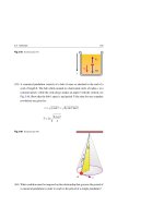
(7) A parallel-plate capacitor has circular plates, each with a radius r = 5 cm.
Assume a vacuum separation d = 1 mm exists between the plates, see Fig. 23.16.
How much charge is stored on each plate of the capacitor when their potential
difference has the value

Fig. 23.16 See Exercise (7)

V = 50 V.

d

r

ΔV

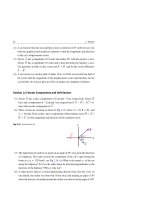
(8) Figure 23.17 shows a set of two parallel sheets of a conductor connected
together to form one plate of a capacitor, while the second set is connected


23.6 Exercises

799

together to form the other plate of the capacitor. Assume that the effective area
of adjacent sheets is A and that the air separation is d. From the figure, confirm
that the number of adjoining sheets of positive and negative charges is 3 and the
capacitor has a capacitance C = 3

◦ A/d.

Fig. 23.17 See Exercise (8)

Area A
1

2

1

2

d

(9) If each set in Exercise 8 consists of n plates, see Fig. 23.18, then show that the
capacitance of the capacitor will be given by:
C=

(2n − 1)
d

Fig. 23.18 See Exercise (9)

1

◦A

2

3

.

.

.

3

.

.

n

Area A
d

1

2

.

n

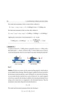
(10) A variable air capacitor used in radio tuning consists of a set of n fixed semicircular plates, each of radius r, and located a distance d from a neighboring
plate of an identical yet rotatable set, see Fig. 23.19. Show that when one set
is rotated by an angle θ, the capacitance is:
C=

(2n − 1) ◦ (π − θ ) r 2
2d


800

23 Capacitors and Capacitance

Fig. 23.19 See Exercise (10)

d

θ
r

(11) A coaxial cable of length = 5 m consists of a solid cylindrical conductor surrounded by a cylindrical conducting shell. The inner conductor has a radius
a = 2.5 mm and carries a charge Q, while the surrounding shell has a radius
b = 8.5 mm and carries a charge −Q, see Fig. 23.20. Assume that Q =
+8 × 10−8 C and that air fills the gap between the conductors. (a) What is
the capacitance of this cable? (b) What is the magnitude of the potential difference between the two cylinders?
Fig. 23.20 See Exercise (11)

−Q

b

a

Q

(12) An isolated spherical conductor carries a charge Q = 4 nC, see Fig. 23.21. The
potential difference between the sphere and its surroundings is V = 100 V.
What is the capacitance formed from the sphere and its surroundings?
Fig. 23.21 See Exercise (12)

Q


23.6 Exercises

801

(13) A capacitor consists of two concentric spheres of radii a = 30 cm and b = 36 cm,
see Fig. 23.22. Assume the gap between the conductors is filled with air. (a)
What is the capacitance of this capacitor? (b) How much charge is stored in the
capacitor if the potential difference between the two spheres is
Fig. 23.22 See Exercise (13)

V = 50 V?

−Q
Q

b

a

(14) Find the capacitance of Earth by assuming that the “missing second conducting
sphere” has an infinite radius. The radius of Earth is R = 6.37 × 106 m.
(15) A spherical drop of mercury has a capacitance of 2.78 f F. If two such drops
combine into one, what would its capacitance be?

Section 23.3 Capacitors with Dielectrics
(16) Two parallel plates of area A = 0.01 m2 are separated by a distance d = 5 ×
10−3 m. The region between these plates is filled with a dielectric material of

κ = 3, and the plates are given equal but opposite charges of 2 µC. (a) What is
the capacitance of this capacitor? (b) Find the potential difference between the
plates.
(17) An air-filled parallel-plate capacitor of 15 µF is connected to a 50 V battery;
then the battery is removed. (a) Find the charge on the capacitor. (b) If the air
is replaced with oil having κ = 2.2, find the new values of the capacitance and
the potential difference between the plates.
(18) A parallel-plate capacitor has an area A = 4 cm2 . (a) Find the maximum stored
charge on the capacitor if air fills the space between the plates. (b) Redo part
(a) when paper is used instead of the air (use the dielectric strengths given in
Table 23.1).


802

23 Capacitors and Capacitance

(19) The charged air capacitor shown in Fig. 23.23 is first placed at a pressure of 1 atm
and found to have a potential difference V = 10,376 V. Then, the capacitor is
placed in a vacuum chamber and the air is removed. The potential difference is

C

-Q

+Q

Air

+Q

V◦ = 10,382 V. Determine the dielectric constant of the air.

C°

-Q

Vacuum

found to rise to

Before
ΔV

After
Δ V°

Fig. 23.23 See Exercise (19)

(20) A parallel-plate capacitor having an area A = 0.2 m2 , and a plate separation
d = 1 mm filled with air as an insulator, is connected to a battery that has
a potential difference V◦ = 12 V, see Fig. 23.24. While the battery is still
connected to the capacitor, a sheet of glass (κ = 4.5) is inserted to fill the space
between the plates, see the figure. (a) Determine both the initial capacitance
(C◦ ) and the initial charge (Q◦ ), then find C and Q after inserting the glass.
(b) If σi is the magnitude of the induced surface charge density on the glass
and σ◦ is the magnitude of the charge density of the plates before the insertion
of the glass, then show that:
σi = (κ − 1)σ◦
(c) Find the values of σi and the induced electric field Ei .

Section 23.4 Capacitors in Parallel and Series
(21) Two capacitors, C1 = 2 µF and C2 = 3 µF, are connected in parallel to a battery
that has a potential difference V = 9 V. (a) Find the equivalent capacitance of
the combination. (b) Find the charge on each capacitor. (c) Find the potential
difference across each capacitor.


23.6 Exercises

803

Fig. 23.24 See Exercise (20)

C°

− Q°

C

+Q

−Q

Glass

+ Q°

Δ V°

Δ V°

B

Before

B

After

(22) The two capacitors of exercise 21 are now connected in series to the same battery
(i.e. with a potential difference V = 9 V). (a) Find the equivalent capacitance
of the combination. (b) Find the charge on each capacitor. (c) Find the potential
difference across each capacitor.
(23) For the combination of capacitors shown in Fig. 23.25, assume that C1 = 1 µF,
C2 = 2 µF, C3 = 3 µF, and V = 6 V. (a) Find the equivalent capacitance of
the combination. (b) Find the charge on each capacitor. (c) Find the potential
difference across each capacitor.
Fig. 23.25 See Exercise (23)

C2
ΔV

C1
C3

(24) Three capacitors, C1 = 6 µF, C2 = 4 µF, and C3 = 12 µF, are connected in four
different ways, as shown in Fig. 23.26. In all configurations, the potential difference is 22 V. How many coulombs of charge pass from the battery to each
combination?
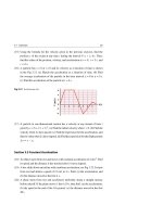
(25) When the three capacitors C1 = 2 µF, C2 = 1 µF, and C3 = 4 µF are connected

to a source of a potential difference V, as shown Fig. 23.27, the charge Q2 on
C2 is found to be 10 µC. (a) Find the values of the charges on the two capacitors
C1 and C3 . (b) Determine the value of V.


804

23 Capacitors and Capacitance

C1

C2

C3

ΔV

Δ V C1

C3

(a)

C1

C2

(b)

ΔV

C2

C1

ΔV C2

C3

C3

(c)

(d)

Fig. 23.26 See Exercise (24)
Fig. 23.27 See Exercise (25)

C1
ΔV
C2

C3

(26) For the circuit shown in Fig. 23.28, C1 = 3 µF, C2 = 6 µF, C3 = 6 µF, C4 =
12 µF, and V = 12 V. (a) Find the equivalent capacitance of the combination.
(b) Find the potential difference across each capacitor.
Fig. 23.28 See Exercise (26)

C1

C3

C2

C4

ΔV

(27) For each of the combinations shown in Fig. 23.29, find a formula that represents
the equivalent capacitance between the terminals A and B.
(28) Assume that in Exercise 27, C = 12 µF and VBA = 12 V. For each combination, find the magnitude of the total charge that the source between A and B
will distribute on the capacitors.


23.6 Exercises

805

C

A

A
C

C

C

C

C

C

C
C

C

A

C

C
A

(a)

B

(b)

C

C

C

B

B

C

C

C

B

(c)

(d)

Fig. 23.29 See Exercise (27)

(29) Two capacitors, C1 = 25 µF and C2 = 40 µF, are charged by being connected to
batteries that have a potential difference V = 50 V, see part (a) of Fig. 23.30.
They are then disconnected from their batteries and connected to each other,
with each positive plate connected to the other’s negative plate; see part (b) of
Fig. 23.30. (a) Find the equivalent capacitance between A and B. (b) What is
the charge Q on the equivalent capacitor? (c) What is the potential difference
VBA between A and B? (d) Find the final charge on each capacitor.

Q1

C1

Q2

C2
Q1 f

C1
Ceq

A

A

B

Q

B

Q2 f

ΔV

ΔV

C2

(a)

(b)

Fig. 23.30 See Exercise (29)

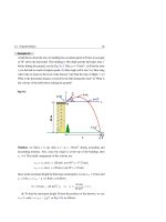
(30) A parallel-plate capacitor has an area A and separation d. A slab of copper of
thickness a is inserted midway between the plates, see part (a) of Fig. 23.31.
Show that the capacitor is equivalent to two capacitors in series, each having a
plate separation (d − a)/2, as shown in part (b) of the figure, and show that the
capacitance after inserting the slab is given by:
C=

◦A

d−a


806

23 Capacitors and Capacitance

Fig. 23.31 See Exercise (30)

A

A
(d-a) / 2

d

Copper

a
(d-a) / 2

(a)

(b)

(31) Show that the capacitance of the capacitor in Fig. 23.10b can be obtained by
finding the equivalent capacitance of two capacitors in series, one capacitor with
a dielectric of thickness a and the second an air-filled capacitor of thickness
d − a.
(32) A parallel-plate capacitor of plate area A and separation d is filled in two different
ways with two dielectrics κ1 and κ2 as shown in parts (a) and (b) of Fig. 23.32.
Show that the capacitances of the two capacitors of parts (a) and (b) are:
C=

◦A

d

κ 1 + κ2
2 ◦ A κ1 κ2
and C =
respectively,
2
d κ1 + κ2

A/2
d

A/2

κ2

κ1

(a)

d

κ1

d/2

κ2

d/2

(b)

Fig. 23.32 See Exercise (32)

Section 23.6 Energy Stored in a charged Capacitor
(33) How much energy is stored in one cubic meter of air due to an electric field of
magnitude 100 V/m?
(34) The two capacitors shown in Fig. 23.33 are uncharged when the switch S is
open. Assume that C1 = 4 µF, C2 = 6 µF, and V = 10 V. The two capacitors
become fully charged when the switch S is closed. (a) Find the energy stored


23.6 Exercises

807

in these two capacitors. (b) Does the stored potential energy in the equivalent
capacitor equal the total stored energy in the two capacitors?
Fig. 23.33 See Exercise (34)

S

ΔV

C1

C2

(35) Redo Example 23.9 when C1 = C2 = 5 µF, and Vi = 10 V. Does the initial
and final stored potential energy remains the same?
(36) A capacitor is charged to a potential difference V. How much should you
increase V so that the stored potential energy is increased by 20%?
(37) Calculate the electric field, the energy density, and the stored potential energy
in the parallel-plate capacitor of Exercise 7.
(38) A parallel-plate capacitor has a capacitance of 4 µF when a mica sheet with
dielectric constant κ = 5 fills the space between the plates. The capacitor is
charged by a battery that has a potential difference 50 V, and is later disconnected. How much work must be done to slowly pull the dielectric from the
capacitor?
(39) For the circuit shown in Fig. 23.34, C1 = 2 µF, C2 = 3 µF, C3 = 6 µF, C4 =
1 µF, and C5 = 2 µF. (a) Find the potential difference between A and B needed
to give C3 a charge of 20 µC. (b) Under these considerations, what is the electric
potential energy stored in the combination?
Fig. 23.34 See Exercise (39)

A
C1
C2

C4

C3

C5
B


808

23 Capacitors and Capacitance

(40) Confirm the relationships shown in Fig. 23.35, where
and

V is shortened by V.

Fixed charge
Before inserting the dielectric

C°

+Q

C°
°

−Q

⇒

°

V°
E°
u°

°

E°

Q (Fixed)

0

κ

Voltmeter

Voltmeter

V°

V

°

⇒

Q°
V° (Fixed)

u°

Fixed charge
After inserting the dielectric
C
+ Q°
− Q°
C
Dielectric
E
Q° (Fixed)

V

0

Fixed voltage
Before inserting the dielectric
C°
+ Q°
− Q°
C°
E

E°

V◦ is shortened by V◦

V°

Fig. 23.35 See Exercise (40)

B

E
u

Fixed voltage
After inserting the dielectric
C
−Q
+Q
C
Dielectric
E
Q

κ

V°

B

Relationships

C = κ C°
Q° (Fixed)
V
V = κ°
E°
κ
u = u ° /κ
E=

Relationships

C = κ C°
Q = κ Q°

V° (Fixed)

V° (Fixed)

E

E = E°

u

u = κ u°


Electric Circuits

24

In this chapter we analyze simple electric circuits that contain devices such as batteries, resistors, and capacitors in various combinations. We begin by introducing
steady-state electric circuits and the concept of a constant rate of flow of electric
charges, known as direct current (dc). We also introduce Kirchhoff’s two rules,
which are used to simplify and analyze more complicated circuits. Finally, we consider circuits containing resistors and capacitors, in which currents can vary with
time.

24.1

Electric Current and Electric Current Density

Electric Current
When there is a net flow of charge across any area, we say there is an electric
current (or simply current) across that area. To maintain a continuous current, we
must maintain a net force on the mobile charge in some way. The net force may
→
result, for example, from an electrostatic field. We assume that an electric field E is
maintained within a conductor such that the charged particle q is acted on by a force
→
F = q E . We refer to this force as the particle’s driving force.
→

To define the current, we consider positive charges moving perpendicularly onto
a surface area A as shown in Fig. 24.1.
Spotlight
The current I across an area A is defined as the net charge flowing perpendicularly to that area per unit time.

H. A. Radi and J. O. Rasmussen, Principles of Physics,
Undergraduate Lecture Notes in Physics, DOI: 10.1007/978-3-642-23026-4_24,

© Springer-Verlag Berlin Heidelberg 2013

809


810

24 Electric Circuits

Thus, if a net charge

Q flows across an area A in a time

t, the average current

Iav across the area is:
Q
t

Iav =

+
+

+

A

+

(24.1)

+
+

A

I
Fig. 24.1 Charged particles in motion perpendicular onto an area A. The current I represents the time
rate of flow of charges and has by convention the direction of the motion of positive charges

When the rate of flow varies with time, we define the instantaneous current (or the
current) I as:
I=

dQ
dt

(24.2)

The SI unit of the current is ampere (abbreviated by A). That is:
1A =

1C
1s

(24.3)

Thus, 1 A is equivalent to 1 C of charge passing through the surface area in 1 s.
Small currents are more conveniently expressed in milliamperes (1 mA = 10−3 A)

or microamperes (1 µA = 10−6 A).
Currents can be due to positive charges, or negative charges, or both. In conductors,
the current is due to the motion of only negatively charged free electrons (called
conduction electrons). By convention, the direction of the current is the direction
of the flow of positive charges. Therefore, the direction of the current is opposite to
the direction of the flow of electrons, see Fig. 24.2b. A moving charge, positive or
negative, is usually referred to as a mobile charge carrier.
+
+

(a)

I1

A

I2

(b)

A

+

-

+

A

I = I1 + I2

(c)

Fig. 24.2 Direction of current due to (a) positive charges, (b) negative charges, and (c) both positive and
negative charges


24.1 Electric Current and Electric Current Density

811

Electric Current Density
The current across an area can be expressed in terms of the motion of the charge carriers. To achieve this we consider a portion of a cylindrical rod that has a cross-sectional
area A, length x, and carries a constant current I, see Fig. 24.3. For convenience we
consider positive charge carriers each having a charge q, and the number of carriers
per unit volume in the rod is n. Therefore, in this portion, the number of carriers is
n A x and the total charge

Q is:
Q = (n A x) q

(24.4)

Fig. 24.3 A portion of a

x

straight rod of uniform
cross-sectional area A,

+

carrying a constant current I.

d

+

A

The mobile charge carriers are

d

+

assumed to be positive and
move with an average speed vd

I

d

d

t

Suppose that all the carriers move with an average speed vd (called the drift speed).
Therefore, during a time interval t, all carriers must achieve a displacement

x = vd t in the x direction. Now, let us choose t such that the carriers in the
cylindrical portion move through a displacement whose magnitude is equal to the
length of the cylinder, see Fig. 24.3. During such a time interval, all the charge carriers in this cylindrical portion must pass through the circular area A at the right end.
Accordingly, we write the last relation as:
Q = (n A vd

t) q

(24.5)

Therefore, the current I = Q/ t in the rod will be given by:
I = n q vd A

(24.6)

The charge carriers in a solid conductor are all free electrons. If the conductor
is isolated, these electrons move with speeds of the order of 106 m/s, and because
of their collisions with the scatterers (atoms or molecules in the conductor), they
move randomly in all directions. This results in a zero drift velocity and hence no net


812

24 Electric Circuits
→

charge transport, which means zero current. When an electric field E is established
→

→

across the conductor, this field exerts an electric force F = −e E on each electron,
producing a current. Of course, the electrons do not move in a straight line along
the conductor, but their resultant motion is complicated and zigzagged, see Fig. 24.4.
Regardless of the collisions of these electrons, they move slowly along the conductor
→
in a direction opposite to E with a drift velocity v→d , see Fig. 24.4.
Fig. 24.4 A schematic

Scatterer

d

Conductor

representation of the random
zigzag motion and the drift of
a free electron with an average

I

-

-

speed vd in a conductor, due to

J

the effect of an external

→

E

electric field E

The current density J is defined as the current per unit area, i.e.:
J=

I
A

(24.7)

Using the relation I = n q vd A, we get:
J = n q vd

(24.8)

where the SI unit of the current density is A/m2 . Equation 24.8 is valid only if J is
uniform and the direction of I is perpendicular to the cross-sectional area A. Generally,
the current density is a vector quantity that has the direction of q v→d , for both signs
of q; that is:
→

J = n q v→d

(24.9)

The amount of current that passes through an element of area dA, can be written

→

→

→

as J • dA , where dA is the vector area of the element. The current that passes
throughout the entire area A is thus:
I=

→

→

J •dA

(24.10)
→

If the current density is uniform across the area and parallel to dA , then this equation
leads to Eq. 24.7.


24.1 Electric Current and Electric Current Density

813

Example 24.1

Estimate the drift speed of the conduction electrons in a copper wire that is 2 mm

in diameter and carries a current of 1 A. Comment on your result. The density of
copper is 8.92 × 103 kg/m3 .
[Hint: Assume that each copper atom contributes one free conduction electron to
the current.]
Solution: To get the drift speed vd , we need to find the free-electron density n.
To get n, we need to know the volume occupied by one kmol of copper. From
the periodic table of elements, see Appendix C, the molar mass of copper is
M(Cu) = 63.546 kg/kmol. Recall that the mass of one kmol of 63.5 Cu contains
Avogadro’s number of atoms (NA = 6.022 × 1026 atoms/kmol). Thus:
Volume of 1 kmol =

Number of copper atoms/m3 =

Mass of 1 kmol
Density

⇒

Avogadro’s number
Volume of 1 kmol

V =

⇒

M
ρ

n=

NA
NA ρ
=
V
M

Therefore:
n =

(6.022 × 1026 atoms/kmol)(8.92 × 103 kg/m3 )
NA ρ
=
M
63.546 kg/kmol

= 8.45 × 1028 atoms/m3
Since the density of free-electrons is equal to the density of copper atoms, then
we use Eq. 24.6 to find the drift speed as follows:
vd =

1 C/s
I
=
ne A
(8.45 × 1028 electrons/m3 )(1.6 × 10−19 C)(π × (10−3 m)2 )

= 2.35 × 10−5 m/s = 8.46 cm/h

(Very small speed)

You might ask why, even though vd is so small, that regular light bulbs light up
very quickly when one turns on its circuit switch? The answer is that the electric
field travels along the connecting wires of the circuit at almost the speed of light,
so electrons everywhere in the wires all begin to drift at once with a small drift
speed.


814

24 Electric Circuits

Example 24.2

One end of the copper wire in example 1 is welded to one end of an aluminum
wire with a 4 mm diameter. The composite wire carries a steady current equal to
that of Example 24.1 (i.e. I = 1 A). (a) What is the current density in each wire?
(b) What is the value of the drift speed vd in the aluminum? [Aluminum has one
free electron per atom and density 2.7 × 103 kg/m3 ]
Solution: (a) Except near the junction, the current density in a copper wire of
radius rCu = 1 mm and aluminum wire of radius rAl = 2 mm are:
I
I
1A
=
=
= 3.18 × 105 A/m2
2
−3 m)2
ACu
π

×
(10
π rCu
I
I
1A
=
=
=
= 7.96 × 104 A/m2
2
AAl
π × (2 × 10−3 m)2
π rAl

JCu =
JAl

(b) From the periodic table of elements, see Appendix C, the molar mass of
aluminum is M(Al) = 26.98 kg/kmol. As in Example 24.1, we find:
n=

NA ρ
(6.022 × 1026 atoms/kmol)(2.7 × 103 kg/m3 )
=
M
26.98 kg/kmol

= 6.03 × 1028 atoms/m3
vd =

1 C/s
I
=
ne A
(6.03 × 1028 electrons/m3 )(1.6 × 10−19 C)(π × (2 × 10−3 m)2 )

= 8.25 × 10−6 m/s = 2.97 cm/h

24.2

Ohm’s Law and Electric Resistance

As a result of maintaining a potential difference
→

→

V across a conductor, an elec-

tric field E and a current density J are established in the conductor. For materials
with electrical properties that are the same in all directions (isotropic materials), the
electric field is found to be proportional to the current density. That is:
→

→

E =ρJ

(Ohm’s law)

(24.11)

where the constant ρ 1 is called the resistivity of the conductor. Materials that obey
this relation are said to obey Ohm’s law:
1

Not to be confused with ρ referring to mass density or charge density.


24.2 Ohm’s Law and Electric Resistance

815

Spotlight
For many materials and most metals, the ratio of the magnitude of the electric
field to the magnitude of the current density is a constant and does not depend
on the electric field producing the current.
→

→

Since it is difficult to measure E and J directly, we need to put Ohm’s law into a
more practical form. This can be obtained by considering a portion of a straight conductor that has a uniform cross-sectional area A and length L, as shown in Fig. 24.5.
In addition, a potential difference V = Vb − Va between the ends of the conductor
(denoted by a and b) will create a straight electric field and current, as also shown in
Fig. 24.5. Since charge carriers in conductors are electrons, they will drift from face
→
a to face b, against the field E .
Fig. 24.5 A potential

L

b

difference V = Vb − Va
across a conductor of
cross-sectional area A and

d

→

q
-

a

e

A

-

length L sets up a field E and
current I

Vb

E

I
J

Va

Recall that for uniform electric fields we have:
V =EL

(24.12)

Using this relation to eliminate E from the scalar form of Eq. 24.11, we get:
V
= ρJ
L

(24.13)

Also, using J = I/A, the potential difference V can be written as:
V = ρ

L
I
A

(24.14)

The quantity in brackets is called the electrical resistance (or simply resistance) of
the conductor and is denoted by the symbol R; that is:
R=ρ

L
A

⇒

R∝ρ

(24.15)


816

24 Electric Circuits

We can define the resistance R as a proportionality constant to the relation V ∝ I
and write the equivalent Ohm’s law as:
Equivalent form

V =IR

of Ohm’s law

The SI unit of resistance is ohm (abbreviated by
=

1

(24.16)

). That is:

1V
1A

(24.17)

This means that if one applies a potential difference of 1 V across a conductor and this
causes 1 A to flow, then the resistance of the conductor is 1 . Note that according to
Eq. 24.15, the SI unit of resistivity is ohm-meter ( .m). Also, since V = Vb − Va ,
we note that the direction of the current is in the direction of decreasing potential.
The inverse of resistivity is called the conductivity σ , thus:
σ =

1
ρ

(24.18)

where the SI unit of σ is ( .m)−1 . The resistance of a conductor can also be written
in terms of the conductivity as follows:
R=

1L
σA

(24.19)

Equations 24.15 and 24.19 hold true only for isotropic conductors. Additionally,
the resistance in Eq. 24.15 depends on the geometry of the resistor through the length

L, area A, and resistivity ρ, which is a constant for a specific metallic conductor
(assuming a constant temperature).
A material obeying Ohm’s law is called an ohmic material or a linear material. If a
material does not obeys Ohm’s law, the material is called a non-ohmic or a nonlinear
material.

Variation of Resistance with Temperature
The variation of resistivity with temperature is mostly linear over a broad range. Since
R ∝ ρ, then for most engineering purposes a good empirical linear approximation
for ρ and R can be written as:
ρ = ρ◦ [1 + α(T − T◦ )]

or

R = R◦ [1 + α(T − T◦ )]

(24.20)


24.2 Ohm’s Law and Electric Resistance

817

where ρ is the resistivity at temperature T (in degrees Celsius), ρ◦ is the resistivity at

a reference temperature T◦ (usually selected to be 20 ◦ C), and α is the temperature
coefficient of resistivity. The same applies for the resistance. The coefficient α is

selected such that Eq. 24.20 matches best with experimental measurements for the
selected range of temperatures. From Eq. 24.20, we find that:

⎧
⎪
⎪
⎨ ρ = ρ − ρ◦
1 R
1 ρ
=
with
α=
(24.21)
R = R − R◦
⎪
ρ◦ T
R◦ T
⎪
⎩ T =T −T
◦

Table 24.1 lists the resistivity ρ and the temperature coefficient of resistivity α
for some materials at 20 ◦ C.
Table 24.1 The resistivity and temperature coefficient of resistivity for various materials at 20◦ Celsius
Material

Resistivity ρ ( .m)

Temperature coefficient of resistivity α [(C◦ )−1 ]

Silver

1.59 × 10−8

3.8 × 10−3

Copper

1.7 × 10−8

3.9 × 10−3

Gold

2.44 × 10−8

3.4 × 10−3

Aluminum

2.82 × 10−8

3.9 × 10−3

Tungsten

5.6 × 10−8

4.5 × 10−3

Iron

10 × 10−8

5.0 × 10−3

Platinum

11 × 10−8

3.98 × 10−3

Lead

22 × 10−8

3.9 × 10−3

Nichromea

1.50 × 10−6

0.4 × 10−3

Carbon

3.5 × 10−5

−0.5 × 10−3

Germanium

0.46

−48 × 10−3

Silicon

640

−75 × 10−3

Glass

1010 –1014

Hard rubber

∼1013

Sulfur

1015

Fused quartz

75 × 1016

a

A nickel–chromium alloy commonly used in heating elements

Most electric circuits use elements called resistors to control the current flowing

through the circuit. Values of the resistance are normally indicated by color-coding
as shown in Tables 24.2 and 24.3.