Giáo trình bài tập luyben cap2
Bạn đang xem bản rút gọn của tài liệu. Xem và tải ngay bản đầy đủ của tài liệu tại đây (967.86 KB, 35 trang )
WILLIAM LUYBEN I
PROCESS MODELING,
SIMULATION
CONTROL
CHEMICAL ENGINEERS
SECOND
I
I
McGraw-Hill Chemical Engineering Series
James J. Carberry,
of Chemical Engineering, University of Notre Dame
James R. Fair, Professor of Chemical Engineering, University of Texas, Austin
P. Schowalter, Professor of Chemical Engineering, Princeton University
Matthew
Professor of Chemical Engineering, University of Minnesota
James
Professor of Chemical Engineering, Massachusetts Institute of Technology
Max S.
Emeritus, Professor of
Engineering, University of Colorado
Building the Literature of a Profession
Fifteen prominent chemical engineers first met in New York more than 60 years
ago to plan a continuing literature for their rapidly growing profession. From
industry came such pioneer practitioners as Leo H. Baekeland, Arthur D. Little,
Charles L. Reese, John V. N. Dorr, M. C. Whitaker, and R. S. McBride. From
the universities came such eminent educators as William H. Walker, Alfred H.
White, D. D. Jackson, J. H. James, Warren K. Lewis, and Harry A. Curtis. H. C.
Parmelee, then editor of Chemical and Metallurgical Engineering, served as chairman and was joined subsequently by S. D. Kirkpatrick as consulting editor.
After several meetings, this committee submitted its report to the
Hill Book Company in September 1925. In the report were detailed specifications
for a correlated series of more than a dozen texts and reference books which have
since become the McGraw-Hill Series in Chemical Engineering and which
became the cornerstone of the chemical engineering curriculum.
From this beginning there has evolved a series of texts surpassing by far the
scope and longevity envisioned by the founding Editorial Board. The
Hill Series in Chemical Engineering stands as a unique historical record of the
development of chemical engineering education and practice. In the series one
finds the milestones of the subject’s evolution: industrial chemistry,
unit operations and processes, thermodynamics, kinetics, and transfer
operations.
Chemical engineering is a dynamic profession, and its literature continues
to evolve. McGraw-Hill and its consulting editors remain committed to a publishing policy that will serve, and indeed lead, the needs of the chemical engineering profession during the years to come.
The Series
Biochemical Engineering Fundamentals
Momentum, Heat, amd Mass Transfer
Optimization: Theory and Practice
Transport Phenomena: A Unified Approach
Chemical and Catalytic Reaction Engineering
Applied Numerical Methods with Personal Computers
Process Systems Analysis and Control
Conceptual Design
Processes
Optimization
Processes
Fundamentals of Transport Phenomena
Nonlinear Analysis in Chemical Engineering
Chemistry of Catalytic Processes
Fundamentals of Multicomponent Distillation
Computer Methods for Solving Dynamic Separation Problems
Handbook of
Natural Gas Engineering
Separation Processes
Process Modeling, Simulation, and Control for Chemical Engineers
Unit Operations of Chemical Engineering
Applied Mathematics in Chemical Engineering
Petroleum Refinery Engineering
Chemical Engineers’ Handbook
Elementary Chemical Engineering
Plant Design and Economics for Chemical Engineers
Synthetic Fuels
The Properties of Gases and Liquids
Process Analysis and Design for Chemical Engineers
Heterogeneous Catalysis in Practice
Mass Transfer
Design of Equilibrium Stage Processes
Chemical Engineering Kinetics
Ness:
to Chemical Engineering Thermodynamics
Mass Transfer Operations
Project Evolution in the Chemical Process Industries
Ness Classical Thermodynamics of Nonelectrolyte Solutions:
with Applications to Phase Equilibria
Distillation
Applied Statistics for Engineers
Reaction Kinetics for Chemical Engineers
The Structure of the Chemical Processing Industries
Conservation of Mass and E
.
Also available from McGraw-Hill
Each outline includes basic theory, definitions, and hundreds of solved
problems and supplementary problems with answers.
Current List Includes:
Advanced Structural Analysis
Basic Equations of Engineering
Descriptive Geometry
Dynamic Structural Analysis
Engineering Mechanics, 4th edition
Fluid Dynamics
Fluid Mechanics
Hydraulics
Introduction to Engineering Calculations
Introductory Surveying
Reinforced Concrete Design, 2d edition
Space Structural Analysis
Statics and Strength of Materials
Strength of Materials, 2d edition
Structural Analysis
Theoretical Mechanics
Available at Your College Bookstore
.
Second Edition
William L. Luyben
Process Modeling and Control Center
Department of Chemical Engineering
University
York St. Louis San Francisco Auckland Bogota Caracas Hamburg
Lisbon London Madrid Mexico Milan Montreal New Delhi
Oklahoma City Paris San Juan
Singapore Sydney Tokyo Toronto
PROCESS MODELING, SIMULATION, AND CONTROL FOR
CHEMICAL ENGINEERS
INTERNATIONAL EDITION 1996
Exclusive rights by McGraw-Hill Book
Singapore for
manufacture and export. This book cannot be m-exported
from the country to which it is consigned by McGraw-Hill.
Copyright
1999, 1973 by McGraw-Hill, Inc.
All rights reserved. Except as permitted under the United States Copyright
Act of 1976, no part of this publication may be reproduced or distributed in
any form or by any means, or stored in a data base or retrieval system,
without the prior written permission of the publisher.
This book was set in Times Roman.
The editors were Lyn Beamesderfer and John M.
The production supervisor was Friederich W.
The cover was designed by John Hite.
Project supervision was done by Harley Editorial Services.
of Congress
Data
William L. Luyben.-2nd ed.
cm.
Bibliography: p.
Includes index.
1. Chemical process-Math
data processing., 3.
1969 ,
When ordering this
use
pro cess
ABOUT THE AUTHOR
William L. Luyben received his B.S. in Chemical Engineering from the Pennsylvania State University where he was the valedictorian of the Class of 1955. He
worked for Exxon for five years at the
Refinery and at the Abadan
Refinery (Iran) in plant. technical service and design of petroleum processing
units. After earning a Ph.D. in 1963 at the University of Delaware, Dr. Luyben
worked for the Engineering Department of DuPont in process dynamics and
control of chemical plants. In 1967 he joined Lehigh University where he is now
Professor of Chemical Engineering and Co-Director of the Process Modeling and
Control Center.
Professor Luyben has published over 100 technical papers and has
authored or coauthored four books. Professor Luyben has directed the theses of
over 30 graduate students. He is an active consultant for industry in the area of
process control and has an international reputation in the field of distillation
column control. He was the recipient of the
Education Award in 1975
and the
Technology Award in 1969 from the Instrument Society
of America.
Overall,
has devoted
to, his profession as a teacher,
researcher, author, and practicing
Robert L.
This book is dedicated to
and Page S. Buckley,
two authentic pioneers
in process modeling
and process control
CONTENTS
Preface
1
1.1
1.2
1.3
1.4
1.5
1.6
Part I
2
Introduction
Examples of the Role of Process Dynamics
and Control
Historical Background
Perspective
Motivation for Studying Process Control
General Concepts
Laws and Languages of Process Control
1.6.1 Process Control Laws
1.6.2 Languages of Process Control
1
6
8
8
11
11
12
Mathematical Models of
Chemical Engineering Systems
Fundamentals
2.1
2.2
1
2.1.1 Uses of Mathematical Models
2.1.2 Scope of Coverage
2.1.3 Principles of Formulation
Fundamental Laws
2.2.1 Continuity Equations
2.2.2 Energy Equation
2.2.3
Equations of Motion
2.2.4 Transport Equations
2.2.5
Equations of State
2.2.6 Equilibrium
2.2.7 Chemical Kinetics
Problems
15
15
15
16
16
17
17
23
27
31
32
33
36
38
PART
MATHEMATICAL
MODELS
OF
CHEMICAL
ENGINEERING
SYSTEMS
I
n the next two chapters we will develop dynamic mathematical models for
several important chemical engineering systems. The examples should illustrate the basic approach to the problem of mathematical modeling.
Mathematical modeling is very much an art. It takes experience, practice,
and brain power to be a good mathematical modeler. You will see a few models
developed in these chapters. You should be able to apply the same approaches to
your own process when the need arises. Just remember to always go back to
basics : mass, energy, and momentum balances applied in their time-varying form.
13
CHAPTER
FUNDAMENTALS
Without doubt, the most important result of developing a mathematical model of
a chemical engineering system is the understanding that is gained of what really
makes the process “tick.” This insight enables you to strip away from the
problem the many extraneous “confusion factors” and to get to the core of the
system. You can see more clearly the cause-and-effect relationships between
the variables.
Mathematical models can be useful in all phases of chemical engineering,
from research and development to plant operations, and even in business and
economic studies.
1. Research and development: determining chemical kinetic mechanisms and
parameters from laboratory or pilot-plant reaction data; exploring the effects
of different operating conditions for optimization and control studies; aiding
in scale-up calculations.
Design: exploring the sizing and arrangement of processing equipment for
dynamic performance; studying the interactions of various parts of the
process, particularly when material recycle or heat integration is used; evaluating alternative process and control structures and strategies; simulating
start-up, shutdown, and emergency situations and procedures.
15
16
MATHEMATICAL
MODELS
OF
CHEMICAL
ENGINEERING
SYSTEMS
3. Plant operation: troubleshooting control and processing problems; aiding in
start-up and operator training; studying the effects of and the requirements for
expansion (bottleneck-removal) projects; optimizing plant operation. It is
usually much cheaper, safer, and faster to conduct the kinds of studies listed
above on a mathematical model than experimentally on an operating unit.
This is not to say that plant tests are not needed. As we will discuss later, they
are a vital part of confirming the validity of the model and of verifying important ideas and recommendations that evolve from the model studies.
We will discuss in this book only deterministic systems that can be described by
ordinary or partial differential equations. Most of the emphasis will be on lumped
systems (with one independent variable, time, described by ordinary differential
equations). Both English and SI units will be used. You need to be familiar with
both.
A. BASIS. The bases for mathematical models are the fundamental physical and
chemical laws, such as the laws of conservation of mass, energy, and momentum.
To study dynamics we will use them in their general form with time derivatives
included.
B. ASSUMPTIONS. Probably the most vital role that the engineer plays in modeling is in exercising his engineering judgment as to what assumptions can be
validly made. Obviously an extremely rigorous model that includes every phenomenon down to microscopic detail would be so complex that it would take a
long time to develop and might be impractical to solve, even on the latest
computers. An engineering compromise between a rigorous description and
getting an answer that is good enough is always required. This has been called
“optimum sloppiness.” It involves making as many simplifying assumptions as
are reasonable without “throwing out the baby with the bath water.” In practice,
this optimum usually corresponds to a model which is as complex as the available computing facilities will permit. More and more this is a personal computer.
The development of a model that incorporates the basic phenomena
occurring in the process requires a lot of skill, ingenuity, and practice. It is an
area where the creativity and innovativeness of the engineer is a key element in
the success of the process.
The assumptions that are made should be carefully considered and listed.
They impose limitations on the model that should always be kept in mind when
evaluating its predicted results.
C. MATHEMATICAL CONSISTENCY OF MODEL. Once all the equations of the
mathematical model have been written, it is usually a good idea, particularly with
big, complex systems of equations, to make sure that the number of variables
equals the number of equations. The so-called “degrees of freedom” of the system
must be zero in order to obtain a solution. If this is not true, the system is
underspecified or overspecified and something is wrong with the formulation of
the problem. This kind of consistency check may seem trivial, but I can testify
from sad experience that it can save many hours of frustration, confusion, and
wasted computer time.
Checking to see that the units of all terms in all equations are consistent is
perhaps another trivial and obvious step, but one that is often forgotten. It is
essential to be particularly careful of the time units of parameters in dynamic
models. Any units can be used (seconds, minutes, hours, etc.), but they cannot be
mixed. We will use “minutes” in most of our examples, but it should be remembered that many parameters are commonly on other time bases and need to be
converted appropriately, e.g., overall heat transfer coefficients in
or
velocity in m/s. Dynamic simulation results are frequently in error because the
engineer has forgotten a factor of “60” somewhere in the equations.
We will concern ourselves in
detail with this aspect of the model in Part II. However, the available solution
techniques and tools must be kept in mind as a mathematical model is developed.
An equation without any way to solve it is not worth much.
An
important but often neglected part of developing a mathematical model is proving that the model describes the real-world situation. At
the design stage this sometimes cannot be done because the plant has not yet
been built. However, even in this situation there are usually either similar existing
plants or a pilot plant from which some experimental dynamic data can be
obtained.
The design of experiments to test the validity of a dynamic model can
sometimes be a real challenge and should be carefully thought out. We will talk
about dynamic testing techniques, such as pulse testing, in Chap. 14.
In this section, some fundamental laws of physics and chemistry are reviewed in
their general time-dependent form, and their application to some simple chemical
systems is illustrated.
The principle of the
conservation of mass when applied to a dynamic system says
MATHEMATICAL MODEL-S OF CHEMICAL ENGINEERING SYSTEMS
The units of this equation are mass per time. Only one total continuity equation
can be written for one system.
The normal steadystate design equation that we are accustomed to using
says that “what goes in, comes out.” The dynamic version of this says the same
thing with the addition of the world “eventually.”
The right-hand side of Eq. (2.1) will be either a partial derivative
or an
ordinary derivative
of the mass inside the system with respect to the independent variable t.
Consider the tank of perfectly mixed liquid shown in Fig. 2.1 into
which flows a liquid stream at a volumetric rate of
or
and with
a density of
or
The volumetric holdup of liquid in the tank is
or
and its density is The volumetric flow rate from the tank is F, and the
density of the outflowing stream is the same as that of the tank’s contents.
The system for which we want to write a total continuity equation is all the
liquid phase in the tank. We call this a macroscopic system, as opposed to a microscopic system, since it is of definite and finite size. The mass balance is around the
whole tank, not just a small, differential element inside the tank.
= time rate of change of
The units of this equation are
or
Since the liquid is perfectly mixed, the density is the same everywhere in the tank; it
does not vary with radial or axial position; i.e., there are no spatial gradients in
density in the tank. This is why we can use a macroscopic system. It also means that
there is only one independent variable,
Since and
are functions only of
an ordinary derivative is used in
(2.2).
2.2. Fluid is flowing through a constant-diameter cylindrical pipe sketched
in Fig. 2.2. The flow is turbulent and therefore we can assume plug-flow conditions,
i.e., each “slice” of liquid flows down the pipe as a unit. There are no radial gradients in velocity or any other properties. However, axial gradients can exist.
Density and velocity can change as the fluid flows along the axial or z direction. There are now two independent variables: time and position z. Density and
FUNDAMENTALS
19
+
FIGURE 2.2
Flow through a pipe.
velocity are functions of both and
and
We want to apply the total
continuity equation [Eq.
to a system that consists of a small slice. The system
is now a “microscopic” one. The differential element is located at an arbitrary spot
z down the pipe. It is
thick and has an area equal to the cross-sectional area of
the pipe A
or
Time rate of change of mass inside system:
at
A dz is the volume of the system; is the density. The units of this equation are
or
Mass flowing into system through boundary at z:
Notice that the units are still
=
Mass flowing out of the system through boundary at z + dz:
The above expression for the flow at z + dz may be thought of as a Taylor series
expansion of a function
around z. The value of the function at a spot dz away
from z is
If the dz is
the series can be truncated after the first derivative term. Letting
=
gives Eq. (2.6).
Substituting these terms into Eq. (2.1) gives
+
1
Canceling out the dz terms and assuming A is constant yield
COMPONENT CONTINUITY EQUATIONS (COMPONENT BALANCES).
Unlike mass, chemical components are not conserved. If a reaction occurs inside
a system, the number of moles of an individual component will increase if it is a
20
MATHEMATICAL
MODELS
OF
CHEMICAL
ENGINEERING
SYSTEMS
product of the reaction or decrease if it is a reactant. Therefore the component
continuity equation of thejth chemical species of the system says
Flow of moles ofjth
component into system
+
flow of moles ofjth
component out of system
1
rate of formation of moles of jth
component from chemical reactions
1
time rate of change of moles of jth
component inside system
1
(2.9)
The units of this equation are moles of component j per unit time.
The flows in and out can be both convective (due to bulk flow) and molecular (due to diffusion). We can write one component continuity equation for each
component in the system. If there are NC components, there are NC component
continuity equations for any one system. However, the one total mass balance
and these NC component balances are not all independent, since the sum of all
the moles times their respective molecular weights equals the total mass. Therefore a given system has only NC independent continuity equations. We usually
use the total mass balance and NC 1 component balances. For example, in a
binary (two-component) system, there would be one total mass balance and one
component balance.
Example 2.3. Consider the same tank of perfectly mixed liquid that we used in
Example 2.1 except that a chemical reaction takes place in the liquid in the tank.
The system is now a CSTR (continuous stirred-tank reactor) as shown in Fig. 2.3.
Component A reacts irreversibly and at a specific reaction rate k to form product,
component B.
A
k
-
B
Let the concentration of component A in the inflowing feed stream be
(moles of
A per unit volume) and in the reactor
Assuming a simple first-order reaction,
the rate of consumption of reactant A per unit volume will be directly proportional
to the instantaneous concentration of A in the tank. Filling in the terms in Eq. (2.9)
for a component balance on reactant A,
Flow of A into system =
Flow of A out of system =
Rate of formation of A from reaction =
P O
The minus sign comes from the fact that A is being consumed, not produced. The
units of all these terms must be the same: moles of A per unit time. Therefore the
term must have these units, for example
of
Thus
the units of k in this system are
Time rate of change of A inside tank =
Combining all of the above gives
dt
=
We have used an ordinary derivative since is the only independent variable in this
lumped system. The units of this component continuity equation are moles of A per
unit time. The left-hand side of the equation is the dynamic term. The first two
terms on the right-hand side are the convective terms. The last term is the generation term.
Since the system is binary (components A and B), we could write another
component continuity equation for component B. Let
be the concentration of B
in moles of B per unit volume.
dt
=
+
Note the plus sign before the generation term since B is being produced by the
reaction. Alternatively we could use the total continuity equation [Eq.
since
,
, and are uniquely related by
(2.11)
where
and
are the molecular weights of components A and B, respectively.
Suppose we have the same macroscopic system as above except that
now consecutive reactions occur. Reactant A goes to B at a specific reaction rate k,,
but B can react at a specific reaction rate
to form a third component C.
c
Assuming first-order reactions, the component continuity equations for components A, B, and C are
dt
dt
dt
(2.12)
MATHEMATICAL
MODELS
OF
CHEMICAL
ENGINEERING
SYSTEMS
The component concentrations are related to the density
(2.13)
Three component balances could be used or we could use two of the component
balances and a total mass balance.
2.5. Instead of fluid flowing down a pipe as in Example 2.2, suppose the
pipe is a tubular reactor in which the same reaction A
B of Example 2.3 takes
place. As a slice of material moves down the length of the reactor the concentration
of reactant
decreases as A is consumed. Density
velocity and concentration
can all vary with time and axial position
We still assume plug-flow conditions
so that there are no radial gradients in velocity, density, or concentration.
The concentration of A fed to the inlet of the reactor at z = 0 is defined as
C
The concentration of A in the reactor
(2.14)
at z =
is defined as
We now want to apply the component continuity equation for reactant A to a small
differential slice of width
as shown in Fig. 2.4. The inflow terms can be split into
two types: bulk flow and diffusion. Diffusion can occur because of the concentration
gradient in the axial direction. It is usually much less important than bulk flow in
most practical systems, but we include it here to see what it contributes to the
model. We will say that the diffusive flux of A,
(moles of A per unit time per unit
area), is given by a Fick’s law type of relationship
where
is a diffusion coefficient due to both diffusion and turbulence in the fluid
flow (so-called “eddy diffusivity”).
has units of length’ per unit time.
The terms in the general component continuity equation [Eq.
are:
Molar flow of A into boundary at z (bulk flow and diffusion)
(moles of
+
Tubular reactor.
FUNDAMENTA LS
23
Molar flow of A leaving system at boundary z + dz
=
+
Rate of formation of A inside system =
+
+
dz
dz
Time rate of change of A inside system =
Substituting into Eq. (2.9) gives
=
+ AN,)
+ AN,)
+ AN, +
+
dz
Adz
+
A
Substituting Eq. (2.16) for
(2.17)
The units of the equation are moles A per volume per time.
2.2.2 Energy Equation
The first law of thermodynamics puts forward the principle of conservation of
energy. Written for a general “open” system (where flow of material in and out of
the system can occur) it is
Flow of internal, kinetic, and
potential energy into system
by convection or diffusion
+
1
flow of internal, kinetic, and
energy out of system
by convection or diffusion
heat added to system by
conduction, radiation, and
reaction
work done by system on
surroundings (shaft work and
PV work)
time rate of change of internal, kinetic,
and potential energy inside system
1
(2.18)
Example 2.6. The CSTR system of Example 2.3 will be considered again, this time
with a cooling coil inside the tank that can remove the exothermic heat of reaction
. mol of A reacted or
mol of A reacted). We use the normal convention
that is negative for an exothermic reaction and positive for an endothermic reaction. The rate of heat generation (energy per time) due to reaction is the rate of
consumption of A times
=
(2.19)
MATHEMATICAL MODELS OF CHEMICAL ENGINEERING
F
CA
FIGURE 2.5
T
CSTR with heat removal.
The rate of heat removal from the reaction mass to the cooling coil is -Q (energy
per time). The temperature of the feed stream is
and the temperature in the
reactor is
or K). Writing Eq. (2.18) for this system,
where
(2.20)
= internal energy (energy per unit mass)
= kinetic energy (energy per unit mass)
= potential energy (energy per unit mass)
= shaft work done by system (energy per time)
P = pressure of system
= pressure of feed stream
Note that all the terms in Eq. (2.20) must have the same units (energy per time) so
the FP terms must use the appropriate conversion factor (778
in English
engineering units).
In the system shown in Fig. 2.5 there is no shaft work, so W = 0. If the inlet
and outlet flow velocities are not very high, the kinetic-energy term is negligible. If
the elevations of the inlet and outlet flows are about the same, the potential-energy
term is small. Thus Eq. (2.20) reduces to
dt
=
+
where
is the specific volume
Enthalpy, H or h, is defined:
+
or
+
+ Q
(2.21)
the reciprocal of the density.
(2.22)
We will use h for the
a liquid stream and H for the enthalpy of a vapor
stream. Thus, for the CSTR, Eq. (2.21) becomes
dt
(2.23)
FUNDAMENTA LS
For liquids the
term is negligible compared to the term, and we use the
time rate of change of the enthalpy of the system instead of the internal energy of
the system.
dt
The enthalpies are functions of composition, temperature, and pressure, but
primarily temperature. From thermodynamics, the heat capacities at constant pressure,
, and at constant volume,
are
(2.25)
To illustrate that the energy is primarily influenced by temperature, let us
simplify the problem by assuming that the liquid enthalpy can be expressed as a
product of absolute temperature and an average heat capacity
or
K) that is constant.
We will also assume that the densities of all the liquid streams are constant. With
these simplifications Eq. (2.24) becomes
d t
=
FT) + Q
(2.26)
2.7. To show what form the energy equation takes for a two-phase system,
consider the CSTR process shown in Fig. 2.6. Both a liquid product stream F and a
vapor product stream
(volumetric flow) are withdrawn from the vessel. The pressure in the reactor is P. Vapor and liquid volumes are
and V. The density and
temperature of the vapor phase are and . The mole fraction of A in the vapor is
y. If the phases are in thermal equilibrium, the vapor and liquid temperatures are
equal (T =
If the phases are in phase equilibrium, the liquid and vapor compositions are related by Raoult’s law, a relative volatility relationship or some other
vapor-liquid equilibrium relationship (see Sec. 2.2.6). The enthalpy of the vapor
phase H
or
is a function of composition y, temperature
and
pressure P. Neglecting kinetic-energy and potential-energy terms and the work term,
Example
T
FIGURE 2.6
Two-phase CSTR with heat removal.
MATHEMATICAL
MODELS
OF
CHEMICAL
ENGINEERING
SYSTEMS
and replacing internal energies with enthalpies in the time derivative, the energy
equation of the system (the vapor and liquid contents of the tank) becomes
dt
=
+Q
(2.27)
In order to express this equation explicitly in terms of temperature, let us
again use a very simple form for
=
and an equally simple form for H.
H=
T+
(2.28)
where
is an average heat of vaporization of the mixture. In a more rigorous
model
could be a function of temperature
composition y, and pressure P.
Equation (2.27) becomes
dt
=
T+
+Q
(2.29)
Example 2.8. To illustrate the application of the energy equation to a microscopic
system, let us return to the plug-flow tubular reactor and now keep track of temperature changes as the fluid flows down the pipe. We will again assume no radial
gradients in velocity, concentration, or temperature (a very poor assumption in
some strongly exothermic systems if the pipe diameter is not kept small). Suppose
that the reactor has a cooling jacket around it as shown in Fig. 2.7. Heat can be
transferred from the process fluid reactants and products at
the
metal wall of the reactor at temperature
The heat is subsequently transferred to
the cooling water. For a complete description of the system we would need energy
equations for the process fluid, the metal wall, and the cooling water. Here we will
concern ourselves only with the process energy equation.
Looking at a little slice of the process fluid as our system, we can derive each
of the terms of Eq. (2.18). Potential-energy and kinetic-energy terms are assumed
negligible, and there is no work term. The simplified forms of the internal energy
and enthalpy are assumed. Diffusive flow is assumed negligible compared to bulk
flow. We will include the possibility for conduction of heat axially along the reactor
due to molecular or turbulent conduction.
FIGURE 2.7
Jacketed tubular reactor.
FUNDAMENTALS
27
Flow of energy (enthalpy) into boundary at z due to bulk flow :
T
lb
with English engineering units of
Btu
lb,,,
= Btu/min
Flow of energy (enthalpy) out of boundary at z +
P
T+
dz
Heat generated by chemical reaction = -A dz
Heat transferred to metal wall =
where
= heat transfer film coefficient,
= diameter of pipe, ft
Heat conduction into boundary at z =
A
where
is a heat flux in the z direction due to conduction. We will use Fourier’s
law to express in terms of a temperature driving force:
=
where
min “R.
is an effective thermal conductivity with English engineering units of
Heat conduction out of boundary at z + dz =
A+
Rate of change of internal energy (enthalpy) of the system =
Combining all the above gives
at
A
(2.31)
As any high school student, knows, Newton’s second law of motion says that
force is equal to mass times acceleration for a system with constant mass M.
(2.32)
where
= force, lbr
M = mass, lb,,,
a = acceleration,
= conversion constant needed when English engineering units are used
to keep units consistent = 32.2 lb,,,
This is the basic relationship that is used in writing the equations of motion for a
system. In a slightly more general form, where mass can vary with time,
(2.33)
where
= velocity in the i direction,
= jth force acting in the i direction
Equation (2.33) says that the time rate of change of momentum in the i direction
(mass times velocity in the i direction) is equal to the net sum of the forces
pushing in the i direction. It can be thought of as a dynamic force balance. Or
more eloquently it is called the conservation ofmomentum.
In the real world there are three directions: y, and z. Thus, three force
balances can be written for any system. Therefore, each system has three equations of motion (plus one total mass balance, one energy equation, and NC 1
component balances).
Instead of writing three equations of motion, it is often more convenient
(and always more elegant) to write the three equations as one vector equation.
We will not use the vector form in this book since all our examples will be simple
one-dimensional force balances. The field of fluid mechanics makes extensive use
of the conservation of momentum.
Example 2.9. The gravity-flow tank system described in Chap. 1 provides a simple
example of the application of the equations of motion to a macroscopic system.
Referring to Fig. 1.1, let the length of the exit line be
(ft) and its cross-sectional
area be A,
The vertical, cylindrical tank has a cross-sectional area of A,
The part of this process that is described by a force balance is the liquid
flowing through the pipe. It will have a mass equal to the volume of the pipe
times the density of the liquid This mass of liquid will have a velocity v
equal
to the volumetric flow divided by the cross-sectional area of the pipe. Remember we
have assumed plug-flow conditions and incompressible liquid, and therefore all the
liquid is moving at the same velocity, more or less like a solid rod. If the flow is
turbulent, this is not a bad assumption.
M=
F
(2.34)
The amount of liquid in the pipe will not change with time, but if we want to change
the rate of outflow, the velocity of the liquid must be changed. And to change the
velocity or the momentum of the liquid we must exert a force on the liquid.
The direction of interest in this problem is the horizontal, since the pipe is
assumed to be horizontal. The force pushing on the liquid at the left end of the pipe
is the hydraulic pressure force of the liquid in the tank.
Hydraulic force =
(2.35)
FUNDAMENTA LS
The units of this force are (in English engineering units):
32.2
32.2 lb,,,
= lb,
where g is the acceleration due to gravity and is 32.2
if the tank is at sea level.
The static pressures in the tank and at the end of the pipe are the same, so we do
not have to include them.
The only force pushing in the opposite direction from right to left and
opposing the flow is the frictional force due to the viscosity of the liquid. If the flow
is turbulent, the frictional force will be proportional to the square of the velocity
and the length of the pipe.
Frictional force =
Substituting these forces into Eq.
(2.36)
we get
1
(2.37)
L
The sign of the frictional force is negative because it acts in the direction opposite
the flow. We have defined left to right as the positive direction.
Example 2.10. Probably the best contemporary example of a variable-mass system
would be the equations of motion for a space rocket whose mass decreases as fuel is
consumed. However, to stick with chemical engineering systems, let us consider the
problem sketched in Fig. 2.8. Petroleum pipelines are sometimes used for transferring several products from one location to another on a batch basis, i.e., one
product at a time. To reduce product contamination at the end of a batch transfer, a
leather ball or “pig” that just fits the pipe is inserted in one end of the line. Inert gas
is introduced behind the pig to push it through the line, thus purging the line of
whatever liquid is in it.
To write a force balance on the liquid still in the pipe as it is pushed out, we
must take into account the changing mass of material. Assume the pig is weightless
and frictionless compared with the liquid in the line. Let z be the axial position of
the pig at any time. The liquid is incompressible (density
and flows in plug flow.
It exerts a frictional force proportional to the square of its velocity and to the length
of pipe still containing liquid.
Frictional force =
Liquid
FIGURE 2.8
Pipeline and pig.
(2.38)