DEPTH ESTIMATION FOR MULTI VIEW VIDEO CODING

VIETNAM NATIONAL UNIVERSITY, HANOI
UNIVERSITY OF ENGINEERING AND TECHNOLOGY

Dinh Trung Anh

DEPTH ESTIMATION FOR MULTI-VIEW VIDEO
CODING

Major: Computer Science

1 - 2015
HA NOI


VIETNAM NATIONAL UNIVERSITY, HANOI
UNIVERSITY OF ENGINEERING AND TECHNOLOGY

Dinh Trung Anh

DEPTH ESTIMATION FOR MULTI-VIEW VIDEO
CODING

Major: Computer Science
Major: Computer Science
Supervisor: Dr. Le Thanh Ha
Supervisor: Dr. BSc.
Co-Supervisor:
Le Thanh
Nguyen
HaMinh Duc
Co-Supervisor: BS. Nguyen Minh Duc

2 – 2015
HA NOI
HA NOI – 2015


AUTHORSHIP
“I hereby declare that the work contained in this thesis is of my own and has not been
previously submitted for a degree or diploma at this or any other higher education
institution. To the best of my knowledge and belief, the thesis contains no materials
previously published or written by another person except where due reference or
acknowledgement is made.”

Signature:………………………………………………

i


SUPERVISOR’S APPROVAL
“I hereby approve that the thesis in its current form is ready for committee examination as
a requirement for the Bachelor of Computer Science degree at the University of
Engineering and Technology.”

Signature:………………………………………………

ii


ACKNOWLEDGEMENT

Firstly, I would like to express my sincere gratitude to my advisers Dr. Le Thanh
Ha of University of Engineering and Technology, Viet Nam National University, Hanoi
and Bachelor Nguyen Minh Duc for their instructions, guidance and their research
experiences.
Secondly, I am grateful to thank all the teachers of University of Engineering and
Technology, VNU for their invaluable lessons which I have learnt during my university
life.
I would like to also thank my friends in K56CA class, University of Engineering
and Technology, VNU.
Last but not least, I greatly appreciate all the help and support that members of
Human Machine Interaction Laboratory of University of Engineering and Technology and
Kotani Laboratory of Japan Advanced Institute of Science and Technology gave me during
this project.
Hanoi, May 8th, 2015

Dinh Trung Anh

iii


ABSTRACT
With the advance of new technologies in the entertainment industry, the FreeViewpoint television (TV), the next generation of 3D medium, is going to give users a
completely new experience of watching TV as they can freely change their viewpoints.
Future TV is going to not only show but also let users “live” inside the 3D scene. A simple
approach for free viewpoint TV is to use current multi-view video technology, which uses
a system of multiple cameras to capture the scene. The views at positions where there is a
lack of camera viewpoints must be synthesized with the support of depth information. This
thesis is to study Depth Estimation Reference Software (DERS) of Moving Pictures Expert
Group (MPEG) which is a reference software for estimating depth from color videos
captured by multi-view cameras. It also provides a method, which uses stored background

information to improve the depth quality taken from the reference software. The
experimental results exhibit the quality improvement of the depth maps estimated from the
proposed method in comparison with those from the traditional method in some cases.

Keywords: Multi-view Video Coding, Depth Estimation Reference Software,
Graph Cut.

iv


TÓM TẮT
Với sự phát triển của công nghệ mới trong ngành công nghiệp giải trí, ti vi góc nhìn
tự do, thế hệ tiếp theo của phương tiện truyền thông, sẽ cho người dùng một trải nghiệm
hoàn toàn mới về ti vi khi họ có thể tự do thay đổi góc nhìn. Ti vi tương lai sẽ không chỉ
hiển thị hình ảnh mà còn cho người dùng “sống” trong khung cảnh 3D. Một hướng tiếp
cận đơn giản cho ti vi đa góc nhìn là sử dụng công nghệ hiện có của video đa góc nhìn với
cả một hệ thống máy quay để chụp lại khung cảnh. Hình ảnh ở các góc nhìn không có
camera phải được tổng hợp với sự hỗ trợ của thông tin độ sâu. Luận văn này sẽ tìm hiểu về
Depth Estimation Reference Software (DERS) của Moving Pictures Expert Group
(MPEG), phần mềm tham khảo để ước lượng độ sâu từ các video màu chụp bởi các máy
quay đa góc nhìn. Đồng thời khóa luận cũng sẽ đưa ra phương pháp mới sử dụng lưu trữ
thông tin nền để cải tiến phần mềm tham khảo. Kết quả thí nghiệm cho thấy sự cái thiện
chất lượng ảnh độ sâu của phương pháp được đề xuất khi so sánh với phương pháp truyền
thống trong một số trường hợp.
Từ khóa: Nén video đa góc nhìn, Phần mềm Ứớc lượng Độ sâu Tham khảo, Cắt
trên Đồ thị

v

CONTENTS

AUTHORSHIP .......................................................................................................... i
SUPERVISOR’S APPROVAL ................................................................................ ii
ACKNOWLEDGEMENT ....................................................................................... iii
ABSTRACT ............................................................................................................ iv
TÓM TẮT ................................................................................................................ v
CONTENTS ............................................................................................................ vi
LIST OF FIGURES ............................................................................................... viii
LIST OF TABLES ................................................................................................... x
ABBREVATIONS .................................................................................................. xi
Chapter 1 .................................................................................................................. 1
INTRODUCTION .................................................................................................... 1
1.1. Introduction and motivation .......................................................................... 1
1.2. Objectives ...................................................................................................... 2
1.3. Organization of the thesis .............................................................................. 3
Chapter 2 .................................................................................................................. 4
DEPTH ESTIMATION REFERENCE SOFTWARE ............................................. 4
2.1. Overview of Depth Estimation Reference Software ..................................... 4
2.2. Disparity - Depth Relation ............................................................................. 8
2.3. Matching cost ................................................................................................. 9
2.3.1. Pixel matching....................................................................................... 10
2.3.2. Block matching ..................................................................................... 10
vi


2.3.3. Soft-segmentation matching ................................................................. 11
2.3.4. Epipolar Search matching ..................................................................... 12
2.4. Sub-pixel Precision ...................................................................................... 13
2.5. Segmentation ............................................................................................... 15

2.6. Graph Cut ..................................................................................................... 16
2.6.1. Energy Function .................................................................................... 16
2.6.2. Optimization.......................................................................................... 18
2.6.3. Temporal Consistency........................................................................... 20
2.6.4. Results ................................................................................................... 21
2.7. Plane Fitting ................................................................................................. 22
2.8. Semi-automatic modes................................................................................. 23
2.8.1. First mode ............................................................................................. 23
2.8.2. Second mode ......................................................................................... 24
2.8.3. Third mode ............................................................................................ 27
Chapter 3 ................................................................................................................ 28
THE METHOD: BACKGROUND ENHANCEMENT ........................................ 28
3.1. Motivation example ..................................................................................... 28
3.2. Details of Background Enhancement .......................................................... 30
Chapter 4 ................................................................................................................ 33
RESULTS AND DISCUSSIONS .......................................................................... 33
4.1. Experiments Setup ....................................................................................... 33
4.2. Results .......................................................................................................... 34
Chapter 5 ................................................................................................................ 38
CONCLUSION ...................................................................................................... 38
REFERENCES ....................................................................................................... 39

vii


LIST OF FIGURES
Figure 1. Basic configuration of FTV system [1]. ................................................... 2
Figure 2. Modules of DERS ..................................................................................... 5
Figure 3. Examples of the relation between disparity and depth of objects............. 7
Figure 4. The disparity is given by the difference 𝑑 = 𝑥𝐿 − 𝑥𝑅, where 𝑥𝐿 is the xcoordinate of the projected 3D coordinate 𝑥𝑃 onto the left camera image plane 𝐼𝑚𝐿 and

𝑥𝑅 is the x-coordinate of the projection onto the right image plane 𝐼𝑚𝑅 [7]. .................... 8
Figure 5. Exampled rectified pair of images from “Poznan_Game” sequence [11].
........................................................................................................................................... 12
Figure 6. Explanation of epipolar line search [11]. ................................................ 13
Figure 7. Matching precisions with searching in horizontal direction only [12] ... 14
Figure 8. Explanation of vertical up-sampling [11]. .............................................. 14
Figure 9. Color reassignment after Segmentation for invisibility. From (a) to (c):
cvPyrMeanShiftFiltering, cvPyrSegmentation and cvKMeans2 [9]. ................................ 15
Figure 10. An example of 𝐺𝛼 for a 1D image. The set of pixels in the image is 𝑉 =
{𝑝, 𝑞, 𝑟, 𝑠} and the current partition is 𝑃 = {𝑃1, 𝑃2, 𝑃𝛼} where 𝑃1 = {𝑝}, 𝑃2 = {𝑞, 𝑟},
and 𝑃𝛼 = {𝑠}. Two auxiliary nodes 𝑎 = 𝑎{𝑝, 𝑞}, 𝑏 = 𝑎{𝑟, 𝑠} are introduced between
neighboring pixels separated in the current partition. Auxiliary nodes are added at the
boundary of sets 𝑃𝑙 [14]. ................................................................................................... 18
Figure 11. Properties of a minimum cut 𝐶 on 𝐺𝛼 for two pixel 𝑝,q such that 𝑑𝑝 ≠
𝑑𝑞. Dotted lines show the edges cut by 𝐶and solid lines show the edges in the induced
graph 𝐺𝐶 = 𝑉, 𝐸 − 𝐶 [14]. ................................................................................................ 20
Figure 12. Depth maps after graph cut: Champagne and BookArrival [9]. ........... 21
Figure 13. Depth maps after Plane Fitting. Left to Right:: cvPyrMeanShiftFiltering,
cvPyrSegmentation and cvKMeans2. Top to bottom: Champagne, BookArrival [9]. ..... 23
Figure 14. Flow chart of the SADERS 1.0 algorithm [17]. ................................... 24
viii


Figure 15. Simplified flow diargram of the second mode of SADERS [18]. ........ 25
Figure 16. Left to right: camera view, automatic depth result, semi-automatic depth
result, manual disparity map, manual edge map. Top to bottom: BookArrival, Champagne,
Newspaper, Doorflowers and BookArrival [18]. .............................................................. 27
Figure 17. Motivation example .............................................................................. 29
Figure 18. Frames of Depth sequence of Pantomime. Figure a and b have been
processed for better visual effect. ...................................................................................... 29

Figure 19. Motion search ........................................................................................ 31
Figure 20. Background Intensity map and Background Depth map ...................... 32
Figure 21. Experiment Setup .................................................................................. 34
Figure 22. Experimental results. Red line: DERS with background enhancement.
Blue line: DERS without background enhancement ......................................................... 35
Figure 23. Failed case in sequence Champagne ..................................................... 37
Figure 24. Comparison frame-to-frame of the Pantomime test. Figure a and b have
been processed for better visual effect. ............................................................................. 37

ix


LIST OF TABLES
Table 1. Weights assigned to edges in Graph Cut. ................................................. 19
Table 2. Average PSNR of experimental results .................................................... 36

x


ABBREVATIONS
DERS

Depth Estimation Reference Software

VSRS

View Synthesis Reference Software

SADERS

Semi-Automatic Depth Estimation Reference Software

FTV

Free viewpoint Television

MVC

Multi-view Video Coding

3DV

3D Video

MPEG

Moving Pictures Expert Group

PSNR

Peak Signal-to-Noise Ratio

HEVC

High Efficiency Video Coding

GC

Graph Cut

xi


Chapter 1

INTRODUCTION

1.1. Introduction and motivation
The concept of free-viewpoint Television (FTV) was first proposed by Nagoya
University at MPEG conference in 2001, focusing on creating a new generation of 3D
medium which allows watchers to freely change their viewpoints [1]. To achieve this goal,
MPEG has been conducting a range of international standardization activities divided into
two phases: Multi-view Video Coding (MVC) and 3D Video (3DV). Multi-view Video
Coding, the first phase of FTV, was started in March 2004 and completed in May 2009,
targeting on the coding part of FTV from the ray captures of multi-view cameras,
compression and transmission of images to synthesis of new views. On the other hand, the
second phase 3DV started in April 2007 was about serving these 3D views on different
types of 3D displays [1].
In the basic configuration of FTV system, as shown in the Figure 1, 3D scene is
fully captured by a multi-camera system. The captured images are, then, corrected to
eliminate “the misalignment and luminance differences of the cameras” [1]. Then,
corresponding to each corrected image, a depth map is estimated. Along with the color
images, these depth maps all are compressed and transmitted to the user side. The idea of
1


calculating the depth maps at sender sides and sending them along with the color images
helps reducing the computational work of the receiver. Moreover, it allows FTV system to
be able to show the infinite number of views based on the finite number of coding views
[2]. After being uncompressed, the depth maps and existing views are used to generate new

views, which fully describe the original 3D scene from any viewpoints which the users
want.

Figure 1. Basic configuration of FTV system [1].
Although depth estimation only works as an intermediate step in the whole coding
process of MVC, it actually is a crucial part, since depth maps are the key idea to interpolate
free viewpoints. In the sequences of MVC standardization activities, Depth Estimation
Reference Software (DERS) was introduced to MPEG as a reference software for
estimating depth maps from sequences of images captured by an array of multiple cameras.
At first, there is only one fully automatic mode in DERS; however, as in many cases, the
inefficiency of depth estimation of the automatic mode of DERS leads to the low quality
of synthesized views, new semi-automatic modes were added to improve the performance
of DERS and the quality of the synthesized views. These new modes, nevertheless, share
a same feature which is that a very good frame having manual support but poor
performance in the next ones.

1.2. Objectives
The objectives of this thesis are about understanding and learning technologies in
the Depth Estimation Reference Software (DERS) of MPEG. Moreover, in this thesis, I
introduce a new method to improve the performance of DERS called background
2


enhancement. The basic idea of this method is storing the background of the scenes and
using them to estimate the separation between the foreground and the background. The
color map and depth map of background are stored overtime from the first frame. Since the
background does not change too much over the sequence, these maps can be used to support
the depth estimation process in DERS.

1.3. Organization of the thesis

Chapter 2 is spent describing the theories, structures, techniques and modes of
DERS. Among them, there is a temporal enhancement method, based on which, I
developed a method to improve the performance of DERS. My method will be described
clearly in Chapter 3. The setup and the results of experiments to compare the method with
the original DERS is illustrated in Chapter 4 along with further discussion. The final
Chapter, Chapter 5, will conclude the overall information of this thesis.

3


Chapter 2

DEPTH ESTIMATION REFERENCE
SOFTWARE

2.1. Overview of Depth Estimation Reference Software
In April 2008, Nagoya University for the first time has proposed the Depth
Estimation Reference Software (DERS) to the 84th MPEG Conference in Archamps,
France in the document [3]. In this document, Nagoya has provided all the specification
and also the usage of DERS. The initial algorithm of DERS, nonetheless, had already been
presented in previous MPEG documents [4] and [5]; it included three steps: a pixel
matching step, a graph cut and a conversion step from disparity to depth. All of these
techniques had already been used for years to estimate depth from stereo cameras.
However, while a stereo camera consists of only two co-axial horizontally aligned cameras,
a multi-view camera system often includes multiple cameras which are arranged as a linear
or circular array. Moreover, the input of DERS is not only color images but also a sequence
of images or a video, which requires a synchronization for the capture time of cameras in
the system. The output of DERS, therefore, is also a sequence which each frame is a depth
map corresponding to a frame of color sequences. Since the first version, many
improvements have been made in order to enhance the quality of depth maps: Sub-pixel

precision at DER1.1, temporal consistency at DERS 2.0, Block Matching and Plane Fitting
at DER 3.0… However, because of the inefficiency of traditional automatic DERS, in
DERS 4.0 and 4.9, semi-automatic modes and then reference mode have been respectively
introduced as alternative approaches. In semi-automatic DERS (or SADERS), manual
4


input files are provided at some specific frames. With the power of temporal enhancement
techniques, the manual information is propagated to next frames to support the depth
estimation process. On the other hand, reference mode takes an existing depth sequence
from another camera as a reference when it estimates a depth map for new views. Until the
latest version of DERS, new techniques have been kept integrating into it to improve the
performance. In July 2014, DERS software manual for DERS 6.1 has been released [6].
Left, right and
center Image

Sub-pixel precision
Segmentation

(Optional)
Depth map of
previous frame

(Optional)
Matching cost
Update error cost

(Optional)

Reference

depth

Manual input

Graph cut

Plane fitting
(Optional)
Post processing
(Optional)
Depth map

Figure 2. Modules of DERS
5


After six versions of DERS have been released, the configuration of DERS has
become more and more intricate with various techniques and methods. Figure 2 shows the
modules and the process of depth estimation of DERS.
As it can be seen from Figure 2, while most of modules are optional, there are still
two modules (matching cost and graph cut) that cannot be replaceable. As mentioned
above, these two modules have existed from the initial version of DERS as the key for
estimating depth. The process of estimating depth starts at each frame in the sequence with
three images: left, center and right images. The center image is actually the frame at the
center camera view and also the image we want to calculate the corresponding depth map.
In order to do so, it is required to have a left image from the camera in the left of the center
camera and a right image from the camera in the right of the center camera. It is also
required that these images are synchronized in the capture time. These images are, then,
passed to an optional sub-pixel precision module, which us interpolation methods to double
or quadruple the size of the left and right images to increase the precision of depth

estimation. The matching cost module, as its name, finds a value to match the pixel of the
center image with those of left or right images. Although there are several methods to
calculate the matching cost, values from these share a same property that the smaller they
are, the higher chance two pixels are matched. These matching values are then modified as
some additional information is added to them before it goes to the graph cut module. A
global energy optimization technique, graph cut, is used to label each pixel to a suitable
depth or disparity based on the matching cost values, additional information and the
smoothness property. Segmentation can also be used to support the graph cut optimization
process as it divides the center image into segments, pixels in each of which are likely to
have the same depth. After the graph cut process, a depth map has already been generated;
however, for better depth quality, the plane fitting and post processing steps can be
optionally used. While the plane fitting method smoothens depth values of pixels in a
segment by considering it as a plane in space, the post processing, which appears only in
the semi-automatic modes, reapplies the manual information into the depth map.

6


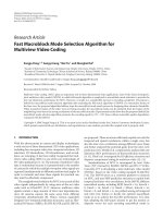
Figure 3. Examples of the relation between disparity and depth of objects
7


2.2. Disparity - Depth Relation
All algorithms to estimate depth for multi-view coding or even for stereo camera
are all based on the relation between depth and disparity. “The term disparity can be looked
upon as horizontal distance between two matching pixels” [7]. The Figure 3Error!
eference source not found. can illustrate this relation. The three images in Figure 3 from
top to bottom are taken respectively from Camera 37, 39 and 41 of Sequence Champagne
of Nagoya University [8]. It can be seen that objects, which are further to the camera
system, tend to move horizontally to the left less than the nearer ones. While the girl and

the table, which is near the capture plane, moves over views, the furthest speaker nearly
stays at its position in both three images. This phenomenon can be explained by camera
pinhole model and mathematics with the Figure 4.

Figure 4. The disparity is given by the difference 𝑑 = 𝑥𝐿 − 𝑥𝑅 , where 𝑥𝐿 is
the x-coordinate of the projected 3D coordinate 𝑥𝑃 onto the left camera image
plane 𝐼𝑚𝐿 and 𝑥𝑅 is the x-coordinate of the projection onto the right image plane
𝐼𝑚𝑅 [7] .
From the Figure 4, [7] has proved that the distance of images of an object (or
disparity) is inversely proportional to the depth of that object:

8


𝑑 = 𝑥𝐿 − 𝑥𝑅 = 𝑓 (

𝑥𝑃 + 𝑙 𝑥𝑃 − 𝑙
2𝑓𝑙
)=
−
𝑧𝑃
𝑧𝑃
𝑧𝑃

(1)

where
𝑑 is the disparity or the distance of images of object-point 𝑃 captured by two
cameras,
𝑥𝐿 , 𝑥𝑅 are the coordinates of images of object-point 𝑃

𝑓 is the focal length of both cameras,
2𝑙 is the distance between two cameras,
𝑧𝑃 is the depth of the object-point 𝑃.

As it was proved that the depth and the disparity of an object is inversely
proportional, the problem of estimating the depth turned into that of calculating the
disparity or finding a matching pixel for each pixels in the center image.

2.3. Matching cost
To calculate the disparity of each pixel in the center image, it is required to match
those pixels with their correspondences in the left and the right images. As mentioned
before, input images of DERS are all corrected to eliminate difference of illumination and
synchronized in capture time. We, therefore, can assume that intensities of matching pixels
of same object-points are almost similar. This assumption is also the key to estimate
matching pixels.
To reduce the complexity of computation, cameras are aligned horizontally.
Moreover, the image sequences are all rectified, which makes the matching pixels align in
a same horizontal level. In other words, instead of looking all over the left or right images
for a single matching pixel, we only need to find it in one horizontal row.

9


Using two mentioned above ideas, matching cost or error cost functions are formed
to help find the matching pixels. They all share the property that the smaller value the
function responds the higher chance it is the matching pixel we are looking for.

2.3.1. Pixel matching
The pixel matching cost function is the simplest matching cost function in DERS.
It appeared in DERS from the initial version introduced by Nagoya University in [4]. For

each pixel in the center image and each disparity in a predefined range, DERS evaluates
matching cost function by calculating the absolute intensity difference between the pixel
in the center image and those in the left and right images respectively and choosing the
minimum value. Therefore, the smaller result is that the more similar intensities of pixels
and the more likely those pixels are matching. For more specific, we have the below
formula:
𝐶 (𝑥, 𝑦, 𝑑 ) = min(𝐶𝐿 (𝑥, 𝑦, 𝑑 ), 𝐶𝑅 (𝑥, 𝑦, 𝑑 )),

(2)

where
𝐶𝐿 (𝑥, 𝑦, 𝑑 ) = |𝐼𝐶 (𝑥, 𝑦) − 𝐼𝐿 (𝑥 + 𝑑, 𝑦)|
𝐶𝑅 (𝑥, 𝑦, 𝑑 ) = |𝐼𝐶 (𝑥, 𝑦) − 𝐼𝑅 (𝑥 − 𝑑, 𝑦)|

2.3.2. Block matching
To improve the performance of DERS, the document [9] presented a new matching
method called block matching. While a pixel matching cost function compares pixel to
pixel, the block matching cost function works with window comparison. For more specific,
when matching two pixels with each other, the block matching method concerns about
comparing windows containing those pixels. The main advantage of this method over the
pixel matching method is that it reduces noise sensitivity. However, this advantage comes
along with a disadvantage, which is loss of detail and more computation when a bigger
window size is selected [7]. DERS, therefore, only uses 3x3 windows with matching pixels
at their center:
10


𝐶 (𝑥, 𝑦, 𝑑 ) = min(𝐶𝐿 (𝑥, 𝑦, 𝑑 ), 𝐶𝑅 (𝑥, 𝑦, 𝑑 )),

(3)

Where
𝑥+1

1
𝐶𝐿 (𝑥, 𝑦, 𝑑 ) = ∑
9

𝑦+1

∑ |𝐼𝑐 (𝑖, 𝑗) − 𝐼𝐿 (𝑖 + 𝑑, 𝑗)|

𝑖=𝑥−1 𝑗=𝑦−1
𝑥+1

1
𝐶𝑅 (𝑥, 𝑦, 𝑑 ) = ∑
9

𝑦+1

∑ |𝐼𝑐 (𝑖, 𝑗) − 𝐼𝑅 (𝑖 − 𝑑, 𝑗)|

𝑖=𝑥−1 𝑗=𝑦−1

For pixels at the corners or edges of images, where the 3x3 windows do not exist,
pixel matching or smaller block matching (2x2, 2x3 or 3x2) are used.

2.3.3. Soft-segmentation matching
Similar to the block matching, soft-segmentation matching method also uses

aggregation windows in comparison [10]. However, each pixel in the block window is
weighted differently by its distance and intensity similarity to the center pixel; this feature
resembles to the bilateral filtering technique [7]. Moreover, the size of window of softsegmentation in DERS can be changed in the configuration file and it is normally quite
large as the default value is 24x24. Soft-segmentation matching, therefore, takes much
more time for computing than block matching and pixel matching. Below is the formula of
soft-segmentation matching cost function:
𝐶 (𝑥, 𝑦, 𝑑 ) = min(𝐶𝐿 (𝑥, 𝑦, 𝑑 ), 𝐶𝑅 (𝑥, 𝑦, 𝑑 )),
where
𝐶𝐿 (𝑥, 𝑦, 𝑑 ) =

∑(𝑖,𝑗)𝜖 𝑤(𝑥,𝑦) 𝑊𝐿 (𝑖, 𝑗, 𝑥, 𝑦)𝑊𝐶 (𝑖 + 𝑑, 𝑗, 𝑥 + 𝑑, 𝑦)|𝐼𝐶 (𝑖, 𝑗) − 𝐼𝐿 (𝑖 + 𝑑, 𝑗)|
∑(𝑖,𝑗)𝜖 𝑤(𝑥,𝑦) 𝑊𝐿 (𝑖, 𝑗, 𝑥, 𝑦)𝑊𝐶 (𝑖 + 𝑑, 𝑗, 𝑥 + 𝑑, 𝑦)

11

(4)


𝐶𝑅 (𝑥, 𝑦, 𝑑 ) =

∑(𝑖,𝑗) 𝜖 𝑤(𝑥,𝑦) 𝑊𝑅 (𝑖, 𝑗, 𝑥, 𝑦)𝑊𝐶 (𝑖 − 𝑑, 𝑗, 𝑥 − 𝑑, 𝑦)|𝐼𝐶 (𝑖, 𝑗) − 𝐼𝑅 (𝑖 − 𝑑, 𝑗)|
∑(𝑖,𝑗) 𝜖 𝑤(𝑥,𝑦) 𝑊𝑅 (𝑖, 𝑗, 𝑥, 𝑦)𝑊𝐶 (𝑖 − 𝑑, 𝑗, 𝑥 − 𝑑, 𝑦)

and
𝑤(𝑥, 𝑦) is a soft-segmentation window center at (𝑥, 𝑦)
𝑊 (𝑖, 𝑗, 𝑥, 𝑦) is the weight function for the pixel (𝑖, 𝑗) in the window centered at
(𝑥, 𝑦):
𝑊 (𝑖, 𝑗, 𝑥, 𝑦) = 𝑒

−

|𝐼(𝑥,𝑦)−𝐼(𝑖,𝑗)| |(𝑥,𝑦)−(𝑖,𝑗)|
−
𝛾𝐶
𝛾𝑑

2.3.4. Epipolar Search matching
As mentioned above, all images are rectified to reduce the complexity in searching
for matching pixels since we only have to make a search in a horizontal line instead of the
whole image. However in document [11], authors from Poznan University of Technology
pointed out that “in the case of sparse or circular camera arrangement”, rectification
“distort the image at unacceptable level” as in Figure 5Error! Reference source not
found..

Figure 5. Exampled rectified pair of images from “Poznan_Game”
sequence [11].
12