Introduction to machine learning www kho sach blogspot com

INTRODUCTION
TO

MACHINE LEARNING
AN EARLY DRAFT OF A PROPOSED
TEXTBOOK

Nils J. Nilsson
Robotics Laboratory
Department of Computer Science
Stanford University
Stanford, CA 94305
e-mail:
December 4, 1996
Copyright c 1997 Nils J. Nilsson
This material may not be copied, reproduced, or distributed without the
written permission of the copyright holder.


Contents
1 Preliminaries

1.1 Introduction : : : : : : : : : : : : : : : :
1.1.1 What is Machine Learning? : : :
1.1.2 Wellsprings of Machine Learning
1.1.3 Varieties of Machine Learning : :
1.2 Learning Input-Output Functions : : : :
1.2.1 Types of Learning : : : : : : : :
1.2.2 Input Vectors : : : : : : : : : : :
1.2.3 Outputs : : : : : : : : : : : : : :
1.2.4 Training Regimes : : : : : : : : :

1.2.5 Noise : : : : : : : : : : : : : : :
1.2.6 Performance Evaluation : : : : :
1.3 Learning Requires Bias : : : : : : : : : :
1.4 Sample Applications : : : : : : : : : : :
1.5 Sources : : : : : : : : : : : : : : : : : :
1.6 Bibliographical and Historical Remarks

2 Boolean Functions

2.1 Representation : : : : : : : : : : : : :
2.1.1 Boolean Algebra : : : : : : : :
2.1.2 Diagrammatic Representations
2.2 Classes of Boolean Functions : : : : :
2.2.1 Terms and Clauses : : : : : : :
2.2.2 DNF Functions : : : : : : : : :
i

:
:
:
:
:
:

:
:
:
:
:
:

:
:
:
:
:
:
:
:
:
:
:
:
:
:
:

:
:
:
:
:
:
:
:
:
:
:
:
:
:

:
:
:
:
:
:
:

:
:
:
:
:
:
:
:
:
:
:
:
:
:
:
:
:
:
:
:
:

:
:
:
:
:
:
:
:
:
:
:
:
:
:
:
:
:
:
:
:
:

:
:
:
:
:
:
:
:

:
:
:
:
:
:
:
:
:
:
:
:
:

:
:
:
:
:
:
:
:
:
:
:
:
:
:
:
:

:
:
:
:
:

:
:
:
:
:
:
:
:
:
:
:
:
:
:
:
:
:
:
:
:
:

:
:

:
:
:
:
:
:
:
:
:
:
:
:
:
:
:
:
:
:
:

:
:
:
:
:
:
:
:
:
:

:
:
:
:
:
:
:
:
:
:
:

:
:
:
:
:
:
:
:
:
:
:
:
:
:
:
:
:
:

:
:
:

:
:
:
:
:
:
:
:
:
:
:
:
:
:
:
:
:
:
:
:
:

1

1
1

3
5
6
6
8
9
9
10
10
10
13
14
15

17

17
17
18
19
19
20


2.2.3 CNF Functions : : : : : : : : : :
2.2.4 Decision Lists : : : : : : : : : : :
2.2.5 Symmetric and Voting Functions
2.2.6 Linearly Separable Functions : :
2.3 Summary : : : : : : : : : : : : : : : : :
2.4 Bibliographical and Historical Remarks

3 Using Version Spaces for Learning
3.1
3.2
3.3
3.4
3.5

Version Spaces and Mistake Bounds : :
Version Graphs : : : : : : : : : : : : : :
Learning as Search of a Version Space :
The Candidate Elimination Method : :
Bibliographical and Historical Remarks

4 Neural Networks

:
:
:
:
:
:
:
:
:
:
:

:
:

:
:
:
:
:
:
:
:
:

:
:
:
:
:
:
:
:
:
:
:

:
:
:
:
:
:
:
:

:
:
:

:
:
:
:
:
:
:
:
:
:
:

:
:
:
:
:
:
:
:
:
:
:

:
:

:
:
:
:
:
:
:
:
:

:
:
:
:
:
:
:
:
:
:
:

:
:
:
:
:
:
:
:

:
:
:

:
:
:
:
:
:
:
:
:
:
:

:
:
:
:
:
:
:
:
:
:
:

4.1 Threshold Logic Units : : : : : : : : : : : : : : : : : : : : :
4.1.1 De nitions and Geometry : : : : : : : : : : : : : : :

4.1.2 Special Cases of Linearly Separable Functions : : : :
4.1.3 Error-Correction Training of a TLU : : : : : : : : :
4.1.4 Weight Space : : : : : : : : : : : : : : : : : : : : : :
4.1.5 The Widrow-Ho Procedure : : : : : : : : : : : : : :
4.1.6 Training a TLU on Non-Linearly-Separable Training
Sets : : : : : : : : : : : : : : : : : : : : : : : : : : :
4.2 Linear Machines : : : : : : : : : : : : : : : : : : : : : : : :
4.3 Networks of TLUs : : : : : : : : : : : : : : : : : : : : : : :
4.3.1 Motivation and Examples : : : : : : : : : : : : : : :
4.3.2 Madalines : : : : : : : : : : : : : : : : : : : : : : : :
4.3.3 Piecewise Linear Machines : : : : : : : : : : : : : : :
4.3.4 Cascade Networks : : : : : : : : : : : : : : : : : : :
4.4 Training Feedforward Networks by Backpropagation : : : :
4.4.1 Notation : : : : : : : : : : : : : : : : : : : : : : : : :
4.4.2 The Backpropagation Method : : : : : : : : : : : : :
4.4.3 Computing Weight Changes in the Final Layer : : :
4.4.4 Computing Changes to the Weights in Intermediate
Layers : : : : : : : : : : : : : : : : : : : : : : : : : :
ii

24
25
26
26
27
28

29

29

31
34
35
37

39

39
39
41
42
45
46
49
50
51
51
54
56
57
58
58
60
62
64


4.4.5 Variations on Backprop : : : : : : : : : : : : : : : :
4.4.6 An Application: Steering a Van : : : : : : : : : : : :
4.5 Synergies Between Neural Network and Knowledge-Based

Methods : : : : : : : : : : : : : : : : : : : : : : : : : : : : :
4.6 Bibliographical and Historical Remarks : : : : : : : : : : :

5 Statistical Learning

5.1 Using Statistical Decision Theory : : : : : : : : : : : :
5.1.1 Background and General Method : : : : : : : :
5.1.2 Gaussian (or Normal) Distributions : : : : : :
5.1.3 Conditionally Independent Binary Components
5.2 Learning Belief Networks : : : : : : : : : : : : : : : :
5.3 Nearest-Neighbor Methods : : : : : : : : : : : : : : : :
5.4 Bibliographical and Historical Remarks : : : : : : : :

6 Decision Trees

6.1 De nitions : : : : : : : : : : : : : : : : : : : : : : : :
6.2 Supervised Learning of Univariate Decision Trees : :
6.2.1 Selecting the Type of Test : : : : : : : : : : :
6.2.2 Using Uncertainty Reduction to Select Tests
6.2.3 Non-Binary Attributes : : : : : : : : : : : : :
6.3 Networks Equivalent to Decision Trees : : : : : : : :
6.4 Over tting and Evaluation : : : : : : : : : : : : : :
6.4.1 Over tting : : : : : : : : : : : : : : : : : : :
6.4.2 Validation Methods : : : : : : : : : : : : : :
6.4.3 Avoiding Over tting in Decision Trees : : : :
6.4.4 Minimum-Description Length Methods : : : :
6.4.5 Noise in Data : : : : : : : : : : : : : : : : : :
6.5 The Problem of Replicated Subtrees : : : : : : : : :
6.6 The Problem of Missing Attributes : : : : : : : : : :
6.7 Comparisons : : : : : : : : : : : : : : : : : : : : : :

6.8 Bibliographical and Historical Remarks : : : : : : :
iii

:
:
:
:
:
:
:
:
:
:
:
:
:
:
:
:

:
:
:
:
:
:
:
:
:
:

:
:
:
:
:
:
:
:
:
:
:
:
:

:
:
:
:
:
:
:
:
:
:
:
:
:
:
:
:

:
:
:
:
:
:
:

:
:
:
:
:
:
:
:
:
:
:
:
:
:
:
:
:
:
:
:
:
:

:

66
67
68
68

69

69
69
71
75
77
77
79

81

81
83
83
84
88
88
89
89
90
91
92

93
94
96
96
96


7 Inductive Logic Programming
7.1
7.2
7.3
7.4
7.5
7.6
7.7

Notation and De nitions : : : : : : : : : : : : : : : : : :
A Generic ILP Algorithm : : : : : : : : : : : : : : : : :
An Example : : : : : : : : : : : : : : : : : : : : : : : : :
Inducing Recursive Programs : : : : : : : : : : : : : : :
Choosing Literals to Add : : : : : : : : : : : : : : : : :
Relationships Between ILP and Decision Tree Induction
Bibliographical and Historical Remarks : : : : : : : : :

:
:
:
:
:
:

:

:
:
:
:
:
:
:

97

99
100
103
107
110
111
114

8 Computational Learning Theory

117

9 Unsupervised Learning

131

8.1 Notation and Assumptions for PAC Learning Theory : : : : 117
8.2 PAC Learning : : : : : : : : : : : : : : : : : : : : : : : : : : 119

8.2.1 The Fundamental Theorem : : : : : : : : : : : : : : 119
8.2.2 Examples : : : : : : : : : : : : : : : : : : : : : : : : 121
8.2.3 Some Properly PAC-Learnable Classes : : : : : : : : 122
8.3 The Vapnik-Chervonenkis Dimension : : : : : : : : : : : : : 124
8.3.1 Linear Dichotomies : : : : : : : : : : : : : : : : : : : 124
8.3.2 Capacity : : : : : : : : : : : : : : : : : : : : : : : : 126
8.3.3 A More General Capacity Result : : : : : : : : : : : 127
8.3.4 Some Facts and Speculations About the VC Dimension129
8.4 VC Dimension and PAC Learning : : : : : : : : : : : : : : 129
8.5 Bibliographical and Historical Remarks : : : : : : : : : : : 130
9.1 What is Unsupervised Learning? : : : : : : : :
9.2 Clustering Methods : : : : : : : : : : : : : : : :
9.2.1 A Method Based on Euclidean Distance
9.2.2 A Method Based on Probabilities : : : :
9.3 Hierarchical Clustering Methods : : : : : : : :
9.3.1 A Method Based on Euclidean Distance
9.3.2 A Method Based on Probabilities : : : :
9.4 Bibliographical and Historical Remarks : : : :
iv

:
:
:
:
:
:
:
:

:

:
:
:
:
:
:
:

:
:
:
:
:
:
:
:

:
:
:
:
:
:
:
:

:
:
:
:

:
:
:
:

:
:
:
:
:
:
:
:

:
:
:
:
:
:
:
:

131
133
133
136
138
138
138

143


10 Temporal-Di erence Learning
10.1
10.2
10.3
10.4
10.5
10.6
10.7
10.8

Temporal Patterns and Prediction Problems :
Supervised and Temporal-Di erence Methods
Incremental Computation of the ( W)i : : :
An Experiment with TD Methods : : : : : :
Theoretical Results : : : : : : : : : : : : : : :
Intra-Sequence Weight Updating : : : : : : :
An Example Application: TD-gammon : : : :
Bibliographical and Historical Remarks : : :

:
:
:
:
:
:
:
:

:
:
:
:
:
:
:
:

:
:
:
:
:
:
:
:

:
:
:
:
:
:
:
:

:
:

:
:
:
:
:
:

11 Delayed-Reinforcement Learning

The General Problem : : : : : : : : : : : : : : : : : :
An Example : : : : : : : : : : : : : : : : : : : : : : : :
Temporal Discounting and Optimal Policies : : : : : :
Q-Learning : : : : : : : : : : : : : : : : : : : : : : : :
Discussion, Limitations, and Extensions of Q-Learning
11.5.1 An Illustrative Example : : : : : : : : : : : : :
11.5.2 Using Random Actions : : : : : : : : : : : : :
11.5.3 Generalizing Over Inputs : : : : : : : : : : : :
11.5.4 Partially Observable States : : : : : : : : : : :
11.5.5 Scaling Problems : : : : : : : : : : : : : : : : :
11.6 Bibliographical and Historical Remarks : : : : : : : :

11.1
11.2
11.3
11.4
11.5

12 Explanation-Based Learning

Deductive Learning : : : : : : : : : : : : : :

Domain Theories : : : : : : : : : : : : : : :
An Example : : : : : : : : : : : : : : : : : :
Evaluable Predicates : : : : : : : : : : : : :
More General Proofs : : : : : : : : : : : : :
Utility of EBL : : : : : : : : : : : : : : : :
Applications : : : : : : : : : : : : : : : : : :
12.7.1 Macro-Operators in Planning : : : :
12.7.2 Learning Search Control Knowledge
12.8 Bibliographical and Historical Remarks : :

12.1
12.2
12.3
12.4
12.5
12.6
12.7

v

:
:
:
:
:
:
:
:
:
:

:
:
:
:
:
:
:
:
:
:

:
:
:
:
:
:
:
:
:
:

:
:
:
:
:
:
:

:
:
:

:
:
:
:
:
:
:
:
:
:

:
:
:
:
:
:
:
:
:
:

:
:
:
:

:
:
:
:
:
:
:
:
:
:
:
:
:
:
:
:
:
:
:
:
:
:
:
:
:

:
:
:
:

:
:
:
:
:
:
:
:
:
:
:
:
:
:
:
:
:
:
:
:
:
:
:
:
:

:
:
:
:

:
:
:
:
:
:
:
:
:
:
:
:
:
:
:
:
:
:
:
:
:
:
:
:
:

145

145
146

148
150
152
153
155
156

159

159
160
161
164
167
167
169
170
171
172
173

175

175
176
178
182
183
183
183

184
186
187


vi


Preface
These notes are in the process of becoming a textbook. The process is quite
un nished, and the author solicits corrections, criticisms, and suggestions
from students and other readers. Although I have tried to eliminate errors,
some undoubtedly remain|caveat lector. Many typographical infelicities
will no doubt persist until the nal version. More material has yet to
be added. Please let me have your suggestions about topics that are too
important to be left out. I hope that future versions will cover Hop eld
nets, Elman nets and other recurrent nets, radial basis functions, grammar
and automata learning, genetic algorithms, and Bayes networks : : :. I am
also collecting exercises and project suggestions which will appear in future
versions.
My intention is to pursue a middle ground between a theoretical textbook and one that focusses on applications. The book concentrates on the
important ideas in machine learning. I do not give proofs of many of the
theorems that I state, but I do give plausibility arguments and citations to
formal proofs. And, I do not treat many matters that would be of practical
importance in applications the book is not a handbook of machine learning practice. Instead, my goal is to give the reader su cient preparation
to make the extensive literature on machine learning accessible.
Students in my Stanford courses on machine learning have already made
several useful suggestions, as have my colleague, Pat Langley, and my teaching assistants, Ron Kohavi, Karl P eger, Robert Allen, and Lise Getoor.

vii

Some of my
plans for
additions and
other
reminders are
mentioned in
marginal notes.


Chapter 1

Preliminaries
1.1 Introduction
1.1.1 What is Machine Learning?
Learning, like intelligence, covers such a broad range of processes that it is
di cult to de ne precisely. A dictionary de nition includes phrases such as
\to gain knowledge, or understanding of, or skill in, by study, instruction,
or experience," and \modi cation of a behavioral tendency by experience."
Zoologists and psychologists study learning in animals and humans. In
this book we focus on learning in machines. There are several parallels
between animal and machine learning. Certainly, many techniques in machine learning derive from the e orts of psychologists to make more precise
their theories of animal and human learning through computational models. It seems likely also that the concepts and techniques being explored by
researchers in machine learning may illuminate certain aspects of biological
learning.
As regards machines, we might say, very broadly, that a machine learns
whenever it changes its structure, program, or data (based on its inputs
or in response to external information) in such a manner that its expected
future performance improves. Some of these changes, such as the addition
of a record to a data base, fall comfortably within the province of other disciplines and are not necessarily better understood for being called learning.

But, for example, when the performance of a speech-recognition machine
improves after hearing several samples of a person's speech, we feel quite
justi ed in that case to say that the machine has learned.

1


CHAPTER 1. PRELIMINARIES

2

Machine learning usually refers to the changes in systems that perform
tasks associated with arti cial intelligence (AI). Such tasks involve recognition, diagnosis, planning, robot control, prediction, etc. The \changes"
might be either enhancements to already performing systems or ab initio
synthesis of new systems. To be slightly more speci c, we show the architecture of a typical AI \agent" in Fig. 1.1. This agent perceives and models
its environment and computes appropriate actions, perhaps by anticipating
their e ects. Changes made to any of the components shown in the gure
might count as learning. Di erent learning mechanisms might be employed
depending on which subsystem is being changed. We will study several
di erent learning methods in this book.
Sensory signals

Goals

Perception

Model
Planning and
Reasoning

Action
Computation

Actions

Figure 1.1: An AI System
One might ask \Why should machines have to learn? Why not design
machines to perform as desired in the rst place?" There are several reasons
why machine learning is important. Of course, we have already mentioned
that the achievement of learning in machines might help us understand how
animals and humans learn. But there are important engineering reasons as
well. Some of these are:


1.1. INTRODUCTION

3

Some tasks cannot be de ned well except by example that is, we
might be able to specify input/output pairs but not a concise relationship between inputs and desired outputs. We would like machines
to be able to adjust their internal structure to produce correct outputs for a large number of sample inputs and thus suitably constrain
their input/output function to approximate the relationship implicit
in the examples.
It is possible that hidden among large piles of data are important
relationships and correlations. Machine learning methods can often
be used to extract these relationships (data mining).
Human designers often produce machines that do not work as well as
desired in the environments in which they are used. In fact, certain
characteristics of the working environment might not be completely
known at design time. Machine learning methods can be used for

on-the-job improvement of existing machine designs.
The amount of knowledge available about certain tasks might be
too large for explicit encoding by humans. Machines that learn this
knowledge gradually might be able to capture more of it than humans
would want to write down.
Environments change over time. Machines that can adapt to a changing environment would reduce the need for constant redesign.
New knowledge about tasks is constantly being discovered by humans.
Vocabulary changes. There is a constant stream of new events in
the world. Continuing redesign of AI systems to conform to new
knowledge is impractical, but machine learning methods might be
able to track much of it.

1.1.2 Wellsprings of Machine Learning
Work in machine learning is now converging from several sources. These
di erent traditions each bring di erent methods and di erent vocabulary
which are now being assimilated into a more uni ed discipline. Here is a
brief listing of some of the separate disciplines that have contributed to
machine learning more details will follow in the the appropriate chapters:

Statistics: A long-standing problem in statistics is how best to use
samples drawn from unknown probability distributions to help decide
from which distribution some new sample is drawn. A related problem


CHAPTER 1. PRELIMINARIES

4

is how to estimate the value of an unknown function at a new point
given the values of this function at a set of sample points. Statistical

methods for dealing with these problems can be considered instances
of machine learning because the decision and estimation rules depend
on a corpus of samples drawn from the problem environment. We
will explore some of the statistical methods later in the book. Details
about the statistical theory underlying these methods can be found
in statistical textbooks such as Anderson, 1958].

Brain Models:

Non-linear elements with weighted inputs
have been suggested as simple models of biological neurons. Networks of these elements have been studied by several researchers including McCulloch & Pitts, 1943, Hebb, 1949,
Rosenblatt, 1958] and, more recently by Gluck & Rumelhart, 1989,
Sejnowski, Koch, & Churchland, 1988]. Brain modelers are interested in how closely these networks approximate the learning phenomena of living brains. We shall see that several important machine
learning techniques are based on networks of nonlinear elements|
often called neural networks. Work inspired by this school is sometimes called connectionism, brain-style computation, or sub-symbolic
processing.

Adaptive Control Theory: Control theorists study the problem
of controlling a process having unknown parameters which must
be estimated during operation. Often, the parameters change during operation, and the control process must track these changes.
Some aspects of controlling a robot based on sensory inputs represent instances of this sort of problem. For an introduction see
Bollinger & Du e, 1988].

Psychological Models: Psychologists have studied the performance
of humans in various learning tasks. An early example is the EPAM
network for storing and retrieving one member of a pair of words when
given another Feigenbaum, 1961]. Related work led to a number of
early decision tree Hunt, Marin, & Stone, 1966] and semantic network Anderson & Bower, 1973] methods. More recent work of this
sort has been in uenced by activities in arti cial intelligence which
we will be presenting.

Some of the work in reinforcement learning can be traced to e orts
to model how reward stimuli in uence the learning of goal-seeking
behavior in animals Sutton & Barto, 1987]. Reinforcement learning
is an important theme in machine learning research.


1.1. INTRODUCTION

5

Arti cial Intelligence: From the beginning, AI research has been

concerned with machine learning. Samuel developed a prominent
early program that learned parameters of a function for evaluating
board positions in the game of checkers Samuel, 1959]. AI researchers
have also explored the role of analogies in learning Carbonell, 1983]
and how future actions and decisions can be based on previous
exemplary cases Kolodner, 1993]. Recent work has been directed
at discovering rules for expert systems using decision-tree methods
Quinlan, 1990] and inductive logic programming Muggleton, 1991,
Lavrac & Dzeroski, 1994]. Another theme has been saving and
generalizing the results of problem solving using explanation-based
learning DeJong & Mooney, 1986, Laird, et al., 1986, Minton, 1988,
Etzioni, 1993].

Evolutionary Models:

In nature, not only do individual animals learn to perform better,
but species evolve to be better t in their individual niches. Since the
distinction between evolving and learning can be blurred in computer

systems, techniques that model certain aspects of biological evolution
have been proposed as learning methods to improve the performance
of computer programs. Genetic algorithms Holland, 1975] and genetic programming Koza, 1992, Koza, 1994] are the most prominent
computational techniques for evolution.

1.1.3 Varieties of Machine Learning
Orthogonal to the question of the historical source of any learning technique
is the more important question of what is to be learned. In this book, we
take it that the thing to be learned is a computational structure of some
sort. We will consider a variety of di erent computational structures:
Functions
Logic programs and rule sets
Finite-state machines
Grammars
Problem solving systems
We will present methods both for the synthesis of these structures from
examples and for changing existing structures. In the latter case, the change


6

CHAPTER 1. PRELIMINARIES

to the existing structure might be simply to make it more computationally
e cient rather than to increase the coverage of the situations it can handle.
Much of the terminology that we shall be using throughout the book is best
introduced by discussing the problem of learning functions, and we turn to
that matter rst.

1.2 Learning Input-Output Functions

We use Fig. 1.2 to help de ne some of the terminology used in describing
the problem of learning a function. Imagine that there is a function, f ,
and the task of the learner is to guess what it is. Our hypothesis about the
function to be learned is denoted by h. Both f and h are functions of a
vector-valued input X = (x1 x2 : : : xi : : : xn ) which has n components.
We think of h as being implemented by a device that has X as input and
h(X) as output. Both f and h themselves may be vector-valued. We
assume a priori that the hypothesized function, h, is selected from a class
of functions H. Sometimes we know that f also belongs to this class or
to a subset of this class. We select h based on a training set, , of m
input vector examples. Many important details depend on the nature of
the assumptions made about all of these entities.

1.2.1 Types of Learning
There are two major settings in which we wish to learn a function. In one,
called supervised learning, we know (sometimes only approximately) the
values of f for the m samples in the training set, . We assume that if we
can nd a hypothesis, h, that closely agrees with f for the members of ,
then this hypothesis will be a good guess for f |especially if is large.
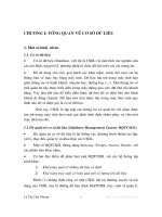
Curve- tting is a simple example of supervised learning of a function.
Suppose we are given the values of a two-dimensional function, f , at the
four sample points shown by the solid circles in Fig. 1.3. We want to t
these four points with a function, h, drawn from the set, H, of second-degree
functions. We show there a two-dimensional parabolic surface above the x1 ,
x2 plane that ts the points. This parabolic function, h, is our hypothesis
about the function, f , that produced the four samples. In this case, h = f
at the four samples, but we need not have required exact matches.
In the other setting, termed unsupervised learning, we simply have a
training set of vectors without function values for them. The problem in
this case, typically, is to partition the training set into subsets, 1 , : : : ,

R , in some appropriate way. (We can still regard the problem as one of


1.2. LEARNING INPUT-OUTPUT FUNCTIONS

7

Training Set:
Ξ = {X1, X2, . . . Xi, . . ., Xm}
x1

X=

.
.
.
xi
.
.
.
xn

h(X)
h

h∈H

Figure 1.2: An Input-Output Function
learning a function the value of the function is the name of the subset
to which an input vector belongs.) Unsupervised learning methods have

application in taxonomic problems in which it is desired to invent ways to
classify data into meaningful categories.
We shall also describe methods that are intermediate between supervised and unsupervised learning.
We might either be trying to nd a new function, h, or to modify an
existing one. An interesting special case is that of changing an existing
function into an equivalent one that is computationally more e cient. This
type of learning is sometimes called speed-up learning. A very simple example of speed-up learning involves deduction processes. From the formulas
A B and B C , we can deduce C if we are given A. From this deductive
process, we can create the formula A C |a new formula but one that
does not sanction any more conclusions than those that could be derived
from the formulas that we previously had. But with this new formula we
can derive C more quickly, given A, than we could have done before. We
can contrast speed-up learning with methods that create genuinely new
functions|ones that might give di erent results after learning than they
did before. We say that the latter methods involve inductive learning. As
opposed to deduction, there are no correct inductions|only useful ones.


CHAPTER 1. PRELIMINARIES

8

sample f-value

h

1500
0
10

1000
00
500
00
0
-10

5
0
-5
-5

0
5

x2

10 -10

x1

Figure 1.3: A Surface that Fits Four Points

1.2.2 Input Vectors
Because machine learning methods derive from so many di erent traditions,
its terminology is rife with synonyms, and we will be using most of them
in this book. For example, the input vector is called by a variety of names.
Some of these are: input vector, pattern vector, feature vector, sample, example, and instance. The components, xi, of the input vector are variously
called features, attributes, input variables, and components.
The values of the components can be of three main types. They might be

real-valued numbers, discrete-valued numbers, or categorical values. As an
example illustrating categorical values, information about a student might
be represented by the values of the attributes class, major, sex, adviser. A
particular student would then be represented by a vector such as: (sophomore, history, male, higgins). Additionally, categorical values may be ordered (as in fsmall, medium, largeg) or unordered (as in the example just
given). Of course, mixtures of all these types of values are possible.
In all cases, it is possible to represent the input in unordered form by
listing the names of the attributes together with their values. The vector
form assumes that the attributes are ordered and given implicitly by a form.
As an example of an attribute-value representation, we might have: (major:
history, sex: male, class: sophomore, adviser: higgins, age: 19). We will be
using the vector form exclusively.
An important specialization uses Boolean values, which can be regarded
as a special case of either discrete numbers (1,0) or of categorical variables


1.2. LEARNING INPUT-OUTPUT FUNCTIONS

9

(True, False).

1.2.3 Outputs
The output may be a real number, in which case the process embodying
the function, h, is called a function estimator, and the output is called an
output value or estimate.
Alternatively, the output may be a categorical value, in which case
the process embodying h is variously called a classi er, a recognizer, or a
categorizer, and the output itself is called a label, a class, a category, or a
decision. Classi ers have application in a number of recognition problems,
for example in the recognition of hand-printed characters. The input in

that case is some suitable representation of the printed character, and the
classi er maps this input into one of, say, 64 categories.
Vector-valued outputs are also possible with components being real
numbers or categorical values.
An important special case is that of Boolean output values. In that
case, a training pattern having value 1 is called a positive instance, and a
training sample having value 0 is called a negative instance. When the input
is also Boolean, the classi er implements a Boolean function. We study the
Boolean case in some detail because it allows us to make important general
points in a simpli ed setting. Learning a Boolean function is sometimes
called concept learning, and the function is called a concept.

1.2.4 Training Regimes
There are several ways in which the training set, , can be used to produce
a hypothesized function. In the batch method, the entire training set is
available and used all at once to compute the function, h. A variation
of this method uses the entire training set to modify a current hypothesis
iteratively until an acceptable hypothesis is obtained. By contrast, in the
incremental method, we select one member at a time from the training set
and use this instance alone to modify a current hypothesis. Then another
member of the training set is selected, and so on. The selection method
can be random (with replacement) or it can cycle through the training set
iteratively. If the entire training set becomes available one member at a
time, then we might also use an incremental method|selecting and using
training set members as they arrive. (Alternatively, at any stage all training
set members so far available could be used in a \batch" process.) Using the
training set members as they become available is called an online method.


10

CHAPTER 1. PRELIMINARIES

Online methods might be used, for example, when the next training instance
is some function of the current hypothesis and the previous instance|as it
would be when a classi er is used to decide on a robot's next action given
its current set of sensory inputs. The next set of sensory inputs will depend
on which action was selected.

1.2.5 Noise
Sometimes the vectors in the training set are corrupted by noise. There are
two kinds of noise. Class noise randomly alters the value of the function
attribute noise randomly alters the values of the components of the input
vector. In either case, it would be inappropriate to insist that the hypothesized function agree precisely with the values of the samples in the training
set.

1.2.6 Performance Evaluation
Even though there is no correct answer in inductive learning, it is important
to have methods to evaluate the result of learning. We will discuss this
matter in more detail later, but, brie y, in supervised learning the induced
function is usually evaluated on a separate set of inputs and function values
for them called the testing set . A hypothesized function is said to generalize
when it guesses well on the testing set. Both mean-squared-error and the
total number of errors are common measures.

1.3 Learning Requires Bias
Long before now the reader has undoubtedly asked why is learning a function possible at all? Certainly, for example, there are an uncountable number of di erent functions having values that agree with the four samples
shown in Fig. 1.3. Why would a learning procedure happen to select the
quadratic one shown in that gure? In order to make that selection we had
at least to limit a priori the set of hypotheses to quadratic functions and

then to insist that the one we chose passed through all four sample points.
This kind of a priori information is called bias, and useful learning without
bias is impossible.
We can gain more insight into the role of bias by considering the special
case of learning a Boolean function of n dimensions. There are 2n di erent
Boolean
inputs possible. Suppose we had no bias that is H is the set of
all 22n Boolean functions, and we have no preference among those that t


1.3. LEARNING REQUIRES BIAS

11

the samples in the training set. In this case, after being presented with one
member of the training set and its value we can rule out precisely one-half
of the members of H|those Boolean functions that would misclassify this
labeled sample. The remaining functions constitute what is called a \version space " we'll explore that concept in more detail later. As we present
more members of the training set, the graph of the number of hypotheses
not yet ruled out as a function of the number of di erent patterns presented
is as shown in Fig. 1.4. At any stage of the process, half of the remaining Boolean functions have value 1 and half have value 0 for any training
pattern not yet seen. No generalization is possible in this case because the
training patterns give no clue about the value of a pattern not yet seen.
Only memorization is possible here, which is a trivial sort of learning.
|Hv| = no. of functions not ruled out
log2|Hv|
2n − j
(generalization is not possible)

2n

0
0

2n
j = no. of labeled
patterns already seen

Figure 1.4: Hypotheses Remaining as a Function of Labeled Patterns Presented
But suppose we limited H to some subset, Hc, of all Boolean functions.
Depending on the subset and on the order of presentation of training patterns, a curve of hypotheses not yet ruled out might look something like the
one shown in Fig. 1.5. In this case it is even possible that after seeing fewer
than all 2n labeled samples, there might be only one hypothesis that agrees
with the training set. Certainly, even if there is more than one hypothesis


CHAPTER 1. PRELIMINARIES

12

remaining, most of them may have the same value for most of the patterns
not yet seen! The theory of Probably Approximately Correct (PAC) learning
makes this intuitive idea precise. We'll examine that theory later.
|Hv| = no. of functions not ruled out
log2|Hv|
2n
depends on order
of presentation
log2|Hc|

0
0

2n
j = no. of labeled
patterns already seen

Figure 1.5: Hypotheses Remaining From a Restricted Subset
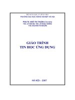
Let's look at a speci c example of how bias aids learning. A Boolean
function can be represented by a hypercube each of whose vertices represents a di erent input pattern. We show a 3-dimensional version in Fig.
1.6. There, we show a training set of six sample patterns and have marked
those having a value of 1 by a small square and those having a value of 0
by a small circle. If the hypothesis set consists of just the linearly separable functions|those for which the positive and negative instances can be
separated by a linear surface, then there is only one function remaining in
this hypothsis set that is consistent with the training set. So, in this case,
even though the training set does not contain all possible patterns, we can
already pin down what the function must be|given the bias.
Machine learning researchers have identi ed two main varieties of bias,
absolute and preference. In absolute bias (also called restricted hypothesisspace bias), one restricts H to a de nite subset of functions. In our example
of Fig. 1.6, the restriction was to linearly separable Boolean functions. In
preference bias, one selects that hypothesis that is minimal according to


1.4. SAMPLE APPLICATIONS

13

x3

x2

x1

Figure 1.6: A Training Set That Completely Determines a Linearly Separable Function
some ordering scheme over all hypotheses. For example, if we had some way
of measuring the complexity of a hypothesis, we might select the one that
was simplest among those that performed satisfactorily on the training set.
The principle of Occam's razor, used in science to prefer simple explanations
to more complex ones, is a type of preference bias. (William of Occam,
1285-?1349, was an English philosopher who said: \non sunt multiplicanda
entia praeter necessitatem," which means \entities should not be multiplied
unnecessarily.")

1.4 Sample Applications
Our main emphasis in this book is on the concepts of machine learning|
not on its applications. Nevertheless, if these concepts were irrelevant to
real-world problems they would probably not be of much interest. As motivation, we give a short summary of some areas in which machine learning
techniques have been successfully applied. Langley, 1992] cites some of the
following applications and others:
a. Rule discovery using a variant of ID3 for a printing industry problem
Evans & Fisher, 1992].


CHAPTER 1. PRELIMINARIES

14

b. Electric power load forecasting using a k-nearest-neighbor rule system
Jabbour, K., et al., 1987].
c. Automatic \help desk" assistant using a nearest-neighbor system

Acorn & Walden, 1992].
d. Planning and scheduling for a steel mill using ExpertEase, a marketed
(ID3-like) system Michie, 1992].
e. Classi cation of stars and galaxies Fayyad, et al., 1993].
Many application-oriented papers are presented at the annual conferences on Neural Information Processing Systems. Among these are papers
on: speech recognition, dolphin echo recognition, image processing, bioengineering, diagnosis, commodity trading, face recognition, music composition, optical character recognition, and various control applications
Various Editors, 1989-1994].
As additional examples, Hammerstrom, 1993] mentions:
a. Sharp's Japanese kanji character recognition system processes 200
characters per second with 99+% accuracy. It recognizes 3000+ characters.
b. NeuroForecasting Centre's (London Business School and University
College London) trading strategy selection network earned an average
annual pro t of 18% against a conventional system's 12.3%.
c. Fujitsu's (plus a partner's) neural network for monitoring a continuous steel casting operation has been in successful operation since
early 1990.
In summary, it is rather easy nowadays to nd applications of machine
learning techniques. This fact should come as no surprise inasmuch as many
machine learning techniques can be viewed as extensions of well known
statistical methods which have been successfully applied for many years.

1.5 Sources
Besides the rich literature in machine learning (a small part of which is referenced in the Bibliography), there are several textbooks that are worth
mentioning Hertz, Krogh, & Palmer, 1991, Weiss & Kulikowski, 1991,
Natarjan, 1991, Fu, 1994, Langley, 1996]. Shavlik & Dietterich, 1990,


1.6. BIBLIOGRAPHICAL AND HISTORICAL REMARKS

15

Buchanan & Wilkins, 1993] are edited volumes containing some of the most
important papers. A survey paper by Dietterich, 1990] gives a good
overview of many important topics. There are also well established conferences and publications where papers are given and appear including:
The Annual Conferences on Advances in Neural Information Processing Systems
The Annual Workshops on Computational Learning Theory
The Annual International Workshops on Machine Learning
The Annual International Conferences on Genetic Algorithms
(The Proceedings of the above-listed four conferences are published
by Morgan Kaufmann.)
The journal Machine Learning (published by Kluwer Academic Publishers).
There is also much information, as well as programs and datasets, available
over the Internet through the World Wide Web.

1.6 Bibliographical and Historical Remarks

To be added.
Every chapter
will contain a
brief survey of
the history of
the material
covered in that
chapter.


16

CHAPTER 1. PRELIMINARIES

Chapter 2

Boolean Functions
2.1 Representation
2.1.1 Boolean Algebra
Many important ideas about learning of functions are most easily presented
using the special case of Boolean functions. There are several important
subclasses of Boolean functions that are used as hypothesis classes for function learning. Therefore, we digress in this chapter to present a review of
Boolean functions and their properties. (For a more thorough treatment
see, for example, Unger, 1989].)
A Boolean function, f (x1 x2 : : : xn ) maps an n-tuple of (0,1) values to
f0 1g. Boolean algebra is a convenient notation for representing Boolean
functions. Boolean algebra uses the connectives , +, and . For example,
the and function of two variables is written x1 x2. By convention, the
connective, \ " is usually suppressed, and the and function is written x1x2 .
x1x2 has value 1 if and only if both x1 and x2 have value 1 if either x1 or x2
has value 0, x1 x2 has value 0. The (inclusive) or function of two variables
is written x1 + x2. x1 + x2 has value 1 if and only if either or both of x1
or x2 has value 1 if both x1 and x2 have value 0, x1 + x2 has value 0. The
complement or negation of a variable, x, is written x. x has value 1 if and
only if x has value 0 if x has value 1, x has value 0.
These de nitions are compactly given by the following rules for Boolean
algebra:
1 + 1 = 1, 1 + 0 = 1, 0 + 0 = 0,
1 1 = 1, 1 0 = 0, 0 0 = 0, and
17