Ebook CMOS VLSI design A circuits and systems perspective (4th edition) Part 2

Combinational
Circuit Design

9

9.1 Introduction
Digital logic is divided into combinational and sequential circuits. Combinational circuits
are those whose outputs depend only on the present inputs, while sequential circuits have
memory. Generally, the building blocks for combinational circuits are logic gates, while
the building blocks for sequential circuits are registers and latches. This chapter focuses on
combinational logic; Chapter 10 examines sequential logic.
In Chapter 1, we introduced CMOS logic with the assumption that MOS transistors
act as simple switches. Static CMOS gates used complementary nMOS and pMOS networks to drive 0 and 1 outputs, respectively. In Chapter 4, we used the RC delay model
and logical effort to understand the sources of delay in static CMOS logic.
In this chapter, we examine techniques to optimize combinational circuits for lower
delay and/or energy. The vast majority of circuits use static CMOS because it is robust,
fast, energy-efficient, and easy to design. However, certain circuits have particularly stringent speed, power, or density restrictions that force another solution. Such alternative
CMOS logic configurations are called circuit families. Section 9.2 examines the most
commonly used alternative circuit families: ratioed circuits, dynamic circuits, and passtransistor circuits. The decade roughly spanning 1994–2004 was the heyday of dynamic
circuits, when high-performance microprocessors employed ever-more elaborate structures to squeeze out the highest possible operating frequency. Since then, power, robustness, and design productivity considerations have eliminated dynamic circuits wherever
possible, although they remain important for memory arrays where the alternatives are
painful. Similarly, other circuit families have been removed or relegated to narrow niches.
Recall from Section 4.3.7 that the delay of a logic gate depends on its output current
I, load capacitance C, and output voltage swing )V
C
(9.1)
)V
I
Faster circuit families attempt to reduce one of these three terms. nMOS transistors provide more current than pMOS for the same size and capacitance, so nMOS networks are
preferred. Observe that the logical effort is proportional to the C/I term because it is
determined by the input capacitance of a gate that can deliver a specified output current.

One drawback of static CMOS is that it requires both nMOS and pMOS transistors on
each input. During a falling output transition, the pMOS transistors add significant capacitance without helping the pulldown current; hence, static CMOS has a relatively large logical effort. Many faster circuit families seek to drive only nMOS transistors with the inputs,
thus reducing capacitance and logical effort. An alternative mechanism must be provided to
tx

327


328

Chapter 9

Combinational Circuit Design

pull the output high. Determining when to pull outputs high involves monitoring the
inputs, outputs, or some clock signal. Monitoring inputs and outputs inevitably loads the
nodes, so clocked circuits are often fastest if the clock can be provided at the ideal time.
Another drawback of static CMOS is that all the node voltages must transition between 0
and VDD. Some circuit families use reduced voltage swings to improve propagation delays
(and power consumption). This advantage must be weighed against the delay and power of
amplifying outputs back to full levels later or the costs of tolerating the reduced swings.
Static CMOS logic is particularly popular because of its robustness. Given the correct
inputs, it will eventually produce the correct output so long as there were no errors in logic
design or manufacturing. Other circuit families are prone to numerous pathologies examined in Section 9.3, including charge sharing, leakage, threshold drops, and ratioing constraints. When using alternative circuit families, it is vital to understand the failure
mechanisms and check that the circuits will work correctly in all design corners.
A host of other circuit families have been proposed, but most have never been used in
commercial products and are doomed to reside on dusty library shelves. Every transistor
contributes capacitance, so most fast structures are simple. Nevertheless, we will describe
some of these circuits in Section 9.4 as a record of ideas that have been explored. A few
hold promise for the future, particularly in specialized applications. Many texts simply catalog these circuit families without making judgments. This book attempts to evaluate the

circuit families so that designers can concentrate their efforts on the most promising ones,
rather than searching for the “gotchas” that were not mentioned in the original papers. Of
course, any such evaluation runs the risk of overlooking advantages or becoming incorrect
as technology changes, so you should use your own judgment.
Silicon-on-insulator (SOI) chips eliminate the conductive substrate. They can achieve
lower parasitic capacitance and better subthreshold slopes, leading to lower power and/or
higher speed, but they have their own special pathologies. Section 9.5 examines considerations for SOI circuits.
CMOS is increasingly applied to ultra-low power systems such as implantable medical devices that require years of operation off of a tiny battery and remote sensors that
scavenge their energy from the environment. Static CMOS gates operating in the subthreshold regime can cut the energy per operation by an order of magnitude at the expense
of several orders of magnitude performance reduction. Section 9.6 explores design issues
for subthreshold circuits.

9.2 Circuit Families
Static CMOS circuits with complementary nMOS pulldown and pMOS pullup networks
are used for the vast majority of logic gates in integrated circuits. They have good noise
margins, and are fast, low power, insensitive to device variations, easy to design, widely
supported by CAD tools, and readily available in standard cell libraries. When noise does
exceed the margins, the gate delay increases because of the glitch, but the gate eventually
will settle to the correct answer. Most design teams now use static CMOS exclusively for
combinational logic. This section begins with a number of techniques for optimizing static
CMOS circuits.
Nevertheless, performance or area constraints occasionally dictate the need for other
circuit families. The most important alternative is dynamic circuits. However, we begin by
considering ratioed circuits, which are simpler and offer a helpful conceptual transition
between static and dynamic. We also consider pass transistors, which had their zenith in
the 1990s for general-purpose logic and still appear in specialized applications.


9.2

Circuit Families

329

9.2.1 Static CMOS
Designers accustomed to AND and OR functions must learn to think in terms of NAND
and NOR to take advantage of static CMOS. In manual circuit design, this is often done
through bubble pushing. Compound gates are particularly useful to perform complex
functions with relatively low logical efforts. When a particular input is known to be latest,
the gate can be optimized to favor that input. Similarly, when either the rising or falling
edge is known to be more critical, the gate can be optimized to favor that edge. We have
focused on building gates with equal rising and falling delays; however, using smaller
pMOS transistors can reduce power, area, and delay. In processes with multiple threshold
voltages, multiple flavors of gates can be constructed with different speed/leakage power
trade-offs.
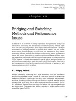
9.2.1.1 Bubble Pushing CMOS stages are inherently inverting, so AND and OR functions must be built from NAND and NOR gates. DeMorgan’s law helps with this conversion:
AšB = A + B

(9.2)

A+B = AšB

These relations are illustrated graphically in Figure 9.1. A NAND gate is equivalent to an
OR of inverted inputs. A NOR gate is equivalent to an AND of inverted inputs. The
same relationship applies to gates with more inputs. Switching between these representations is easy to do on a whiteboard and is often called bubble pushing.

Example 9.1
FIGURE 9.1 Bubble pushing

Design a circuit to compute F = AB + CD using NANDs and NORs.

with DeMorgan’s law

SOLUTION: By inspection, the circuit consists of two ANDs and an OR, shown in Figure

9.2(a). In Figure 9.2(b), the ANDs and ORs are converted to basic CMOS stages. In
Figure 9.2(c and d), bubble pushing is used to simplify the logic to three NANDs.
A
B

A
B
F

F

C
D

C
D

(a)

(b)

A
B

A

B
F

F

C
D

C
D

(c)

(d)

FIGURE 9.2 Bubble pushing to convert ANDs and ORs to NANDs and NORs

9.2.1.2 Compound Gates As described in Section 1.4.5, static CMOS also efficiently
handles compound gates computing various inverting combinations of AND/OR functions in a single stage. The function F = AB + CD can be computed with an AND-ORINVERT-22 (AOI22) gate and an inverter, as shown in Figure 9.3.

A
B
C
D

F

FIGURE 9.3 Logic using AOI22
gate

330

Chapter 9

Combinational Circuit Design

In general, logical effort of compound gates can be different for different inputs. Figure 9.4 shows how logical efforts can be estimated for the AOI21, AOI22, and a more
complex compound AOI gate. The transistor widths are chosen to give the same drive as a
unit inverter. The logical effort of each input is the ratio of the input capacitance of that
input to the input capacitance of the inverter. For the AOI21 gate, this means the logical
effort is slightly lower for the OR terminal (C) than for the two AND terminals (A, B).
The parasitic delay is crudely estimated from the total diffusion capacitance on the output
node by summing the sizes of the transistors attached to the output.

Unit Inverter

AOI21

Y=A

A

Y

Y

A

1

Y

4 B
C

4
4

A

2

B

2

C

Y
1

Complex AOI

Y=A·B+C·D

A
B
C

A
2

AOI22

Y=A·B+C

A
B
C
D

Y = A · (B +C) + D · E

Y

D
E
A
B
C

Y

A

4 B

4

B

6

C

4 D

4

C

6

A

3

A

2 C

2

D

6

E

6

B

2 D

2

E

2

A

2

D

2

2

C

Y

B

gA = 3/3

gA = 6/3

gA = 6/3

gA = 5/3

p = 3/3

gB = 6/3

gB = 6/3

gB = 8/3

gC = 5/3

gC = 6/3

gC = 8/3

p = 7/3

gD = 6/3

gD = 8/3

p = 12/3

gE = 8/3

Y
2

p = 16/3

FIGURE 9.4 Logical efforts and parasitic delays of AOI gates

Example 9.2
Calculate the minimum delay, in Y, to compute F = AB + CD using the circuits from
Figure 9.2(d) and Figure 9.3. Each input can present a maximum of 20 Q of transistor
width. The output must drive a load equivalent to 100 Q of transistor width. Choose
transistor sizes to achieve this delay.
SOLUTION: The path electrical effort is H = 100/20 = 5 and the branching effort is B =
1. The design using NAND gates has a path logical effort of G = (4/3) × (4/3) = 16/9
and parasitic delay of P = 2 + 2 = 4. The design using the AOI22 and inverter has a
path logical effort of G = (6/3) × 1 = 2 and a parasitic delay of P = 12/3 + 1 = 5.
Both designs have N = 2 stages. The path efforts F = GBH are 80/9 and 10, respectively. The path delays are NF 1/N + P, or 10.0 Y and 11.3 Y, respectively. Using compound gates does not always result in faster circuits; simple 2-input NAND gates can
be quite fast.
To compute the sizes, we determine the best stage efforts, fˆ = F 1/ N = 3.0 and 3.2,
respectively. These are in the range of 2.4–6 so we know the efforts are reasonable and


9.2

331

Circuit Families

the design would not improve too much by adding or removing stages. The input capacitance of the second gate is determined by the capacitance transformation
C in =

i

C out × g i
i
fˆ

For the NAND design,
C in =

100 Q × ( 4 / 3)
= 44 Q
3.0

For the AOI22 design,
C in =

100 Q × (1)
= 31 Q
3.2

The paths are shown in Figure 9.5 with transistor widths rounded to integer values.

9.2.1.3 Input Ordering Delay Effect The logical
A
10 B
10
effort and parasitic delay of different gate inputs
10
A
are often different. Some logic gates, like the

B
22
10
22
AOI21 in the previous section, are inherently asymY
22
metric in that one input sees less capacitance than
10 D
C
10
22
another. Other gates, like NANDs and NORs, are
C
10
nominally symmetric but actually have slightly difD
ferent logical effort and parasitic delays for the dif10
ferent inputs.
Figure 9.6 shows a 2-input NAND gate annoFIGURE 9.5 Paths with transistor widths
tated with diffusion parasitics. Consider the falling
output transition occurring when one input held a stable 1 value and the other rises from 0
to 1. If input B rises last, node x will initially be at VDD – Vt ~ VDD because it was pulled up
through the nMOS transistor on input A. The Elmore delay is (R/2)(2C) + R(6C) = 7RC
= 2.33 Y .1 On the other hand, if input A rises last, node x will initially be at 0 V because it
was discharged through the nMOS transistor on input B. No charge must be delivered to
node x, so the Elmore delay is simply R(6C) = 6RC = 2 Y.
In general, we define the outer input to be the input closer to the supply rail (e.g., B)
and the inner input to be the input closer to the output (e.g., A). The parasitic delay is
smallest when the inner input switches last because the intermediate nodes have already
been discharged. Therefore, if one signal is known to arrive later than the others, the gate
is fastest when that signal is connected to the inner input.

Table 8.7 lists the logical effort and parasitic delay for each input of various NAND
gates, confirming that the inner input has a lower parasitic delay. The logical efforts are
lower than initial estimates might predict because of velocity saturation. Interestingly, the
inner input has a slightly higher logical effort because the intermediate node x tends to
rise and cause negative feedback when the inner input turns ON (see Exercise 9.5)
[Sutherland99]. This effect is seldom significant to the designer because the inner input
remains faster over the range of fanouts used in reasonable circuits.

1

Recall that Y = 3RC is the delay of an inverter driving the gate of an identical inverter.

A

13 B

C

13 D

13

21

A

7 C

7

10

B

7 D

7

2

13

2

A

2

B

2x

Y
6C
2C

FIGURE 9.6 NAND gate
delay estimation

Y

332

Chapter 9

A
reset

Combinational Circuit Design

Y

(a)
2

1
A

Y

4/3
4

reset
(b)

FIGURE 9.7 Resettable
buffer optimized for data
input

9.2.1.4 Asymmetric Gates When one input is far less critical than another, even nominally symmetric gates can be made asymmetric to favor the late input at the expense of the
early one. In a series network, this involves connecting the early input to the outer transistor and making the transistor wider so that it offers less series resistance when the critical
input arrives. In a parallel network, the early input is connected to a narrower transistor to
reduce the parasitic capacitance.
For example, consider the path in Figure 9.7(a). Under ordinary conditions, the path
acts as a buffer between A and Y. When reset is asserted, the path forces the output low. If
reset only occurs under exceptional circumstances and can take place slowly, the circuit
should be optimized for input-to-output delay at the expense of reset. This can be done
with the asymmetric NAND gate in Figure 9.7(b). The pulldown resistance is R/4 +
R/(4/3) = R, so the gate still offers the same driver as a unit inverter. However, the capacitance on input A is only 10/3, so the logical effort is 10/9. This is better than 4/3, which is
normally associated with a NAND gate. In the limit of an infinitely large reset transistor
and unit-sized nMOS transistor for input A, the logical effort approaches 1, just like an
inverter. The improvement in logical effort of input A comes at the cost of much higher
effort on the reset input. Note that the pMOS transistor on the reset input is also shrunk.
This reduces its diffusion capacitance and parasitic delay at the expense of slower response
to reset.
CMOS transistors are usually velocity saturated, and thus series transistors carry more
current than the long-channel model would predict. The current can be predicted by collapsing the series stack into an equivalent transistor, as discussed in Section 4.4.6.3. For
asymmetric gates, the equivalent width is that of the inner (narrower) transistor. The
equivalent length increases by the sum of the reciprocals of the relative widths. The relative current is computed using EQ (4.28), where N is the equivalent length.

Example 9.3
Size the nMOS transistors in the asymmetric NAND gate for unit pulldown current
considering velocity saturation. Make the noncritical transistor three times as wide as
the critical transistor. Assume VDD = 1.0 V and Vt = 0.3 V. Use Ec L = 1.04 V for
nMOS devices. Estimate the logical effort of the gate.
SOLUTION: The equivalent length is 1 + 1/3 = 4/3 times that of a unit transistor. Apply2

2

A

1

1

B

1

1

Y

FIGURE 9.8 Perfectly
symmetric 2-input
NAND gate

ing EQ (4.28) gives a relative current of 0.83. Therefore, the transistors’ widths should
be 1.20 and 3.60 to deliver unit current. The logical effort is (1.20 + 2) / 3 = 1.07,
which is even better than predicted without velocity saturation.
In other circuits such as arbiters, we may wish to build gates that are perfectly symmetric so neither input is favored. Figure 9.8 shows how to construct a symmetric NAND
gate.
9.2.1.5 Skewed Gates In other cases, one input transition is more important than the
other. In Section 2.5.2, we defined HI-skew gates to favor the rising output transition and
LO-skew gates to favor the falling output transition. This favoring can be done by decreasing
the size of the noncritical transistor. The logical efforts for the rising (up) and falling (down)
transitions are called gu and gd, respectively, and are the ratio of the input capacitance of the
skewed gate to the input capacitance of an unskewed inverter with equal drive for that transition. Figure 9.9(a) shows how a HI-skew inverter is constructed by downsizing the nMOS

9.2

Circuit Families

333

transistor. This maintains the same effective resistance for
HI-skew
Unskewed Inverter
Unskewed Inverter
Inverter
(equal rise resistance)
(equal fall resistance)
the critical transition while reducing the input capacitance
relative to the unskewed inverter of Figure 9.9(b), thus
2
2
1
reducing the logical effort on that critical transition to gu =
A
Y
A
Y
A
Y
2.5/3 = 5/6. Of course, the improvement comes at the
1/2
1

1/2
expense of the effort on the noncritical transition. The logical effort for the falling transition is estimated by compar(a)
(b)
(c)
ing the inverter to a smaller unskewed inverter with equal
FIGURE 9.9 Logical effort calculation for HI-skew inverter
pulldown current, shown in Figure 9.9(c), giving a logical
effort of gd = 2.5/1.5 = 5/3. The degree of skewing (e.g.,
the ratio of effective resistance for the fast transition relative to the slow transition) impacts
the logical efforts and noise margins; a factor of two is common. Figure 9.10 catalogs HIskew and LO-skew gates with a skew factor of two. Skewed gates are sometimes denoted
with an H or an L on their symbol in a schematic.
Inverter

NAND2

2
A
1

Y
gu = 1
gd = 1
gavg = 1

A

2

B

2

2
A

Y
1/2 g
u = 5/6
gd = 5/3
gavg = 5/4

1

B

1

1

LO-skew

A
1

Y
gu = 4/3
gd = 2/3
gavg = 1

2

B

2

1

1

B

4

A

4

gu = 5/3
gd = 5/3
gavg = 5/3

Y

1

A

4

1/2

gu = 1
gd = 2
gavg = 3/2
Y

1

4

A

Y

2

A

B

gu = 4/3
gd = 4/3
gavg = 4/3
Y

2

HI-skew

2

Y

2

Unskewed

NOR2

1/2

B

2

A

2

gu = 3/2
gd = 3
gavg = 9/4

Y
gu = 2
gd = 1
gavg = 3/2

1

1

FIGURE 9.10 Catalog of skewed gates

Alternating HI-skew and LO-skew gates can be used when only one transition is
important [Solomatnikov00]. Skewed gates work particularly well with dynamic circuits,
as we shall see in Section 9.2.4.
9.2.1.6 P/N Ratios Notice in Figure 9.10 that the average logical effort of the LO-skew
NOR2 is actually better than that of the unskewed gate. The pMOS transistors in the
unskewed gate are enormous in order to provide equal rise delay. They contribute input
capacitance for both transitions, while only helping the rising delay. By accepting a slower
rise delay, the pMOS transistors can be downsized to reduce input capacitance and average
delay significantly.
In general, what is the best P/N ratio for logic gates (i.e., the ratio of pMOS to nMOS
transistor width)? You can prove in Exercise 9.13 that the ratio giving lowest average delay is

gu = 2
gd = 1
gavg = 3/2


334

Chapter 9

Combinational Circuit Design

the square root of the ratio that gives equal rise and fall delays. For processes with a mobility
ratio of Rn/Rp = 2 as we have generally been assuming, the best ratios are shown in Figure
9.11.
Inverter

NAND2
2

Fastest
P/N Ratio

A

1.414
Y
1
gu = 1.14
gd = 0.80
gavg = 0.97

NOR2

2
Y

A

2

B

2

B

2

A

2
Y

gu = 4/3
gd = 4/3
gavg = 4/3

1

1

gu = 2
gd = 1
gavg = 3/2

FIGURE 9.11 Gates with P/N ratios giving least delay

Reducing the pMOS size from 2 to 2 ~ 1.4 for the inverter gives the theoretical
fastest average delay, but this delay improvement is only 3%. However, this significantly
reduces the pMOS transistor area. It also reduces input capacitance, which in turn reduces
power consumption. Unfortunately, it leads to unequal delay between the outputs. Some
paths can be slower than average if they trigger the worst edge of each gate. Excessively
slow rising outputs can also cause hot electron degradation. And reducing the pMOS size
also moves the switching point lower and reduces the inverter’s noise margin.
In summary, the P/N ratio of a library of cells should be chosen on the basis of area,

power, and reliability, not average delay. For NOR gates, reducing the size of the pMOS
transistors significantly improves both delay and area. In most standard cell libraries, the
pitch of the cell determines the P/N ratio that can be achieved in any particular gate.
Ratios of 1.5–2 are commonly used for inverters.
9.2.1.7 Multiple Threshold Voltages Some CMOS processes offer two or more threshold voltages. Transistors with lower threshold voltages produce more ON current, but also
leak exponentially more OFF current. Libraries can provide both high- and low-threshold
versions of gates. The low-threshold gates can be used sparingly to reduce the delay of
critical paths [Kumar94, Wei98]. Skewed gates can use low-threshold devices on only the
critical network of transistors.
VGG
R
Y

Y

Y

9.2.2 Ratioed Circuits

Ratioed circuits depend on the proper size or resistance of
devices for correct operation. For example, in the 1970s and
early 1980s before CMOS technologies matured, circuits were
(a)
(b)
(c)
often built with only nMOS transistors, as shown in Figure
FIGURE 9.12 nMOS ratioed gates
9.12. Conceptually, the ratioed gate consists of an nMOS pulldown network and some pullup device called the static load.
When the pulldown network is OFF, the static load pulls the output to 1. When the pulldown network turns ON, it fights the static load. The static load must be weak enough
that the output pulls down to an acceptable 0. Hence, there is a ratio constraint between

the static load and pulldown network. Stronger static loads produce faster rising outputs,
but increase VOL, degrade the noise margin, and burn more static power when the output
should be 0. Unlike complementary circuits, the ratio must be chosen so the circuit operates correctly despite any variations from nominal component values that may occur
Inputs

Inputs

f

Inputs

f

f


9.2

Circuit Families

during manufacturing. CMOS logic eventually displaced nMOS logic because the static
power became unacceptable as the number of gates increased. However, ratioed circuits
are occasionally still useful in special applications.
A resistor is a simple static load, but large resistors consume a large layout area in typical MOS processes. Another technique is to use an nMOS transistor with the gate tied to
VGG. If VGG = VDD, the nMOS transistor will only pull up to VDD – Vt. Worse yet, the
threshold is increased by the body effect. Thus, using VGG > VDD was attractive. To eliminate this extra supply voltage, some nMOS processes offered depletion mode transistors.
These transistors, indicated with the thick bar, are identical to ordinary enhancement mode
transistors except that an extra ion implantation was performed to create a negative threshold voltage. The depletion mode pullups have their gate wired to the source so Vgs = 0 and
the transistor is always weakly ON.
9.2.2.1 Pseudo-nMOS Figure 9.13(a) shows a pseudo-nMOS inverter. Neither high-value

resistors nor depletion mode transistors are readily available as static loads in most CMOS
Ids (+A)
1000
800

1.8

600

1.5
P = 24

Vin
1.2

400
Load

P = 14

P
200

Ids

0.9

P=4

Vout

0.6

0

16
Vin

0

0.3

0.6

(b)

(a)

0.9

1.2

1.5

1.8

Vout

Ids (+A)
1.8

500

1.5

400

1.2

P = 24

P = 14

300

P = 24

Vout 0.9
200
0.6
P = 14
0.3

0

0
0
(c)

P=4

100

P=4

0.3

0.6

0.9
Vin

1.2

1.5

0

1.8
(d)

FIG 9.13 Pseudo-nMOS inverter and DC transfer characteristics

0.3

0.6

0.9
Vin

1.2

1.5

1.8

335


336

Chapter 9

Combinational Circuit Design

processes. Instead, the static load is built from a single pMOS transistor that has its gate
grounded so it is always ON. The DC transfer characteristics are derived by finding Vout
for which Idsn = |Idsp| for a given Vin, as shown in Figure 9.13(b–c) for a 180 nm process.
The beta ratio affects the shape of the transfer characteristics and the VOL of the inverter.
Larger relative pMOS transistor sizes offer faster rise times but less sharp transfer characteristics. Figure 9.13(d) shows that when the nMOS transistor is turned on, a static DC
current flows in the circuit.
Figure 9.14 shows several pseudo-nMOS logic gates. The pulldown network is like
that of an ordinary static gate, but the pullup network has been replaced with a single
pMOS transistor that is grounded so it is always ON. The pMOS transistor widths are
selected to be about 1/4 the strength (i.e., 1/2 the effective width) of the nMOS pulldown
network as a compromise between noise margin and speed; this best size is process-dependent, but is usually in the range of 1/3 to 1/6.

Inverter

2/3

Y
A

4/3

NAND2
gu = 4/3
gd = 4/9
gavg = 8/9
pu = 18/9
pd = 6/9
pavg = 12/9

2/3
Y
A

8/3

B

8/3

NOR2
gu = 8/3
gd = 8/9
gavg = 16/9
pu = 30/9
pd = 10/9
pavg = 20/9

Generic

2/3
Y
A

4/3 B

4/3

gu = 4/3
gd = 4/9
gavg = 8/9
pu = 30/9
pd = 10/9
pavg = 20/9

Y
Inputs
f

FIGURE 9.14 Pseudo-nMOS logic gates

To calculate the logical effort of pseudo-nMOS gates, suppose a complementary
CMOS unit inverter delivers current I in both rising and falling transitions. For the
widths shown, the pMOS transistors produce I/3 and the nMOS networks produce 4I/3.
The logical effort for each transition is computed as the ratio of the input capacitance to
that of a complementary CMOS inverter with equal current for that transition. For the
falling transition, the pMOS transistor effectively fights the nMOS pulldown. The output

current is estimated as the pulldown current minus the pullup current, (4I/3 – I/3) = I.
Therefore, we will compare each gate to a unit inverter to calculate gd. For example, the
logical effort for a falling transition of the pseudo-nMOS inverter is the ratio of its input
capacitance (4/3) to that of a unit complementary CMOS inverter (3), i.e., 4/9. gu is three
times as great because the current is 1/3 as much.
The parasitic delay is also found by counting output capacitance and comparing it to
an inverter with equal current. For example, the pseudo-nMOS NOR has 10/3 units of
diffusion capacitance as compared to 3 for a unit-sized complementary CMOS inverter, so
its parasitic delay pulling down is 10/9. The pullup current is 1/3 as great, so the parasitic
delay pulling up is 10/3.
As can be seen, pseudo-nMOS is slower on average than static CMOS for NAND
structures. However, pseudo-nMOS works well for NOR structures. The logical effort is
independent of the number of inputs in wide NORs, so pseudo-nMOS is useful for fast
wide NOR gates or NOR-based structures like ROMs and PLAs when power permits.


9.2

337

Circuit Families

Pseudo-nMOS

Example 9.4

In1

Design a k-input AND gate with DeMorgan’s law using static CMOS
inverters followed by a k-input pseudo-nMOS NOR, as shown in Figure

9.15. Let each inverter be unit-sized. If the output load is an inverter of
size H, determine the best transistor sizes in the NOR gate and estimate
the average delay of the path.

1
Y

H

1

Ink

FIGURE 9.15 k-input AND gate
driving load of H

SOLUTION: The path electrical effort is H and the branching effort is B = 1.
The inverter has a logical effort of 1. The pseudo-nMOS NOR has an
average logical effort of 8/9 according to Figure 9.14. The path logical
effort is G = 1 × (8/9) = 8/9, so the path effort is 8H/9. Each stage should
bear an effort of fˆ = 8 H / 9 . Using the capacitance transformation gives
NOR pulldown transistor widths of

C in =

gC out (8 / 9)H
=
=
fˆ
8H / 9

8H
3

unit-sized inverters. As a unit inverter has three units of input capacitance,
the NOR transistor nMOS widths should be 8H . According to Figure
9.14, the pullup transistor should be half this width. The complete circuit
marked with nMOS and pMOS widths is drawn in Figure 9.16.
We estimate the average parasitic delay of a k-input pseudo-nMOS
NOR to be (8k + 4)/9. The total delay in Y is
4 2
D = Nfˆ + P =
3

8 k + 13
H +
9

2

Pseudo-nMOS

2H

1
2

8H

1

FIGURE 9.16 k-input AND
marked with transistor widths

Increasing the number of inputs only impacts the parasitic delay, not the
effort delay.
Pseudo-nMOS gates will not operate correctly if VOL > VIL of the receiving
gate. This is most likely in the SF design corner where nMOS transistors are
weak and pMOS transistors are strong. Designing for acceptable noise margin in
the SF corner forces a conservative choice of weak pMOS transistors in the normal corner. A biasing circuit can be used to reduce process sensitivity, as shown in
Figure 9.17. The goal of the biasing circuit is to create a Vbias that causes P 2 to
deliver 1/3 the current of N 2, independent of the relative mobilities of the
pMOS and nMOS transistors. Transistor N 2 has width of 3/2 and hence produces current 3I/2 when ON. Transistor N1 is tied ON to act as a current source
with 1/3 the current of N2, i.e., I/2. P1 acts as a current mirror using feedback to
establish the bias voltage sufficient to provide equal current as N 1, I/2. The size
of P1 is noncritical so long as it is large enough to produce sufficient current and
is equal in size to P 2. Now, P 2 ideally also provides I/2. In summary, when A is
low, the pseudo-nMOS gate pulls up with a current of I/2. When A is high, the
pseudo-nMOS gate pulls down with an effective current of (3I/2 – I/2) = I. To
first order, this biasing technique sets the relative currents strictly by transistor
widths, independent of relative pMOS and nMOS mobilities.

To other
pseudo-nMOS
gates
P1

Vbias

2

2
1/2
N1

A

P2

Y
gu = 1
3/2
N2 gd = 1/2
gavg = 3/4

FIGURE 9.17 Replica biasing
of pseudo-nMOS gates


338

Chapter 9

en
Y
A

B

C

FIGURE 9.18 PseudonMOS gate with enabled
pullup

Combinational Circuit Design

Such replica biasing permits the 1/3 current ratio rather than the conservative 1/4
ratio in the previous circuits, resulting in lower logical effort. The bias voltage Vbias can be
distributed to multiple pseudo-nMOS gates. Ideally, Vbias will adjust itself to keep VOL
constant across process corners. Unfortunately, the currents through the two pMOS transistors do not exactly match because their drain voltages are unequal, so this technique still
has some process sensitivity. Also note that this bias is relative to VDD, so any noise on
either the bias voltage line or the VDD supply rail will impact circuit performance.
Turning off the pMOS transistor can reduce power when the logic is idle or during
IDDQ test mode (see Section 15.6.4), as shown in Figure 9.18.

Example 9.5
Calculate the static power dissipation of a 32-word × 48-bit ROM that contains a 5:32
pseudo-nMOS row decoder and pMOS pullups on the 48-bit lines. The pMOS transistors have an ON current of 360 RA/Rm and are minimum width (100 nm). VDD =
1.0 V. Assume one of the word lines and 50% of the bitlines are high at any given time.
SOLUTION: Each pMOS transistor dissipates 360 RA/Rm × 0.1 Rm × 1.0 V = 36 RW of
power when the output is low. We expect to see 31 wordlines and 24 bitlines low, so the
total static power is 36 RW × (31 + 24) = 1.98 mW.

9.2.2.2 Ganged CMOS Figure 9.19 illustrates pairs of
CMOS inverters ganged together. The truth table is given
Y
Y
in Table 9.1, showing that the pair compute the NOR funcgu = 1
4/3
4/3

B
gd = 2/3
tion. Such a circuit is sometimes called a symmetric 2 NOR
N1
N2
gavg = 5/6
[ Johnson88], or more generally, ganged CMOS [Schultz90].
(a)
(b)
When one input is 0 and the other 1, the gate can be viewed
FIGURE 9.19 Symmetric 2-input NOR gate
as a pseudo-nMOS circuit with appropriate ratio constraints. When both inputs are 0, both pMOS transistors
turn on in parallel, pulling the output high faster than they would in an ordinary pseudonMOS gate. Moreover, when both inputs are 1, both pMOS transistors turn OFF, saving
static power dissipation. As in pseudo-nMOS, the transistors are sized so the pMOS are
about 1/4 the strength of the nMOS and the pulldown current matches that of a unit
inverter. Hence, the symmetric NOR achieves both better performance and lower power
dissipation than a 2-input pseudo-nMOS NOR.

A

A

P1
2/3 B

P2
2/3

TABLE 9.1 Operation of symmetric NOR
A

B

N1

P1

N2

P2

Y

0
0
1
1

0
1
0
1

OFF
OFF
ON
ON

ON
ON

OFF
OFF

OFF
ON
OFF
ON

ON
OFF
ON
OFF

1
~0
~0
0

Johnson also showed that symmetric structures can be used for NOR gates with more
inputs and even for NAND gates (see Exercises 9.23–9.24). The 3-input symmetric NOR
also works well, but the logical efforts of the other structures are unattractive.
2

Do not confuse this use of symmetric with the concept of symmetric and asymmetric gates from Section
9.2.1.4.


9.2

339

Circuit Families

9.2.3 Cascode Voltage Switch Logic
Cascode Voltage Switch Logic (CVSL3) [Heller84] seeks the benefits of ratioed
circuits without the static power consumption. It uses both true and complementary input signals and computes both true and complementary outputs
using a pair of nMOS pulldown networks, as shown in Figure 9.20(a). The
pulldown network f implements the logic function as in a static CMOS gate,
while f uses inverted inputs feeding transistors arranged in the conduction
complement. For any given input pattern, one of the pulldown networks will be
ON and the other OFF. The pulldown network that is ON will pull that output low. This low output turns ON the pMOS transistor to pull the opposite
output high. When the opposite output rises, the other pMOS transistor turns
OFF so no static power dissipation occurs. Figure 9.20(b) shows a CVSL
AND/NAND gate. Observe how the pulldown networks are complementary,
with parallel transistors in one and series in the other. Figure 9.20(c) shows a
4-input XOR gate. The pulldown networks share A and A transistors to reduce
the transistor count by two. Sharing is often possible in complex functions, and
systematic methods exist to design shared networks [Chu86].
CVSL has a potential speed advantage because all of the logic is performed with nMOS transistors, thus reducing the input capacitance. As in
pseudo-nMOS, the size of the pMOS transistor is important. It fights the
pulldown network, so a large pMOS transistor will slow the falling transition.
Unlike pseudo-nMOS, the feedback tends to turn off the pMOS, so the outputs will settle eventually to a legal logic level. A small pMOS transistor is
slow at pulling the complementary output high. In addition, the CVSL gate
requires both the low- and high-going transitions, adding more delay. Contention current during the switching period also increases power consumption.
Pseudo-nMOS worked well for wide NOR structures. Unfortunately,
CVSL also requires the complement, a slow tall NAND structure. Therefore,
CVSL is poorly suited to general NAND and NOR logic. Even for symmetric
structures like XORs, it tends to be slower than static CMOS, as well as more
power-hungry [Chu87, Ng96]. However, the ideas behind CVSL help us
understand dual-rail domino and complementary pass-transistor logic discussed in later sections.

9.2.4 Dynamic Circuits

Y

Y

Inputs

f

f

(a)
Y= A · B

Y= A · B
A

A

B

B

(b)

Y

Y

D

D

D

C

C

C

B

B

B

A

A

(c)

FIGURE 9.20 CVSL gates

2/3

2
A

1
(a)

φ

1

A

1

Y

Y
A
(b)

4/3

Y

(c)

Ratioed circuits reduce the input capacitance by replacing the pMOS transis- FIGURE 9.21 Comparison of (a) static
tors connected to the inputs with a single resistive pullup. The drawbacks of CMOS, (b) pseudo-nMOS, and (c) dynamic
ratioed circuits include slow rising transitions, contention on the falling transi- inverters
tions, static power dissipation, and a nonzero VOL. Dynamic circuits circumvent these drawbacks by using a clocked pullup transistor rather than a pMOS that is
always ON. Figure 9.21 compares (a) static CMOS, (b) pseudo-nMOS, and (c) dynamic
inverters. Dynamic circuit operation is divided into two modes, as shown in Figure 9.22.
During precharge, the clock K is 0, so the clocked pMOS is ON and initializes the output

Y high. During evaluation, the clock is 1 and the clocked pMOS turns OFF. The output
may remain high or may be discharged low through the pulldown network. Dynamic
3

Many authors call this circuit family Differential Cascode Voltage Switch Logic (DCVS [Chu86] or DCVSL
[Ng96]). The term cascode comes from analog circuits where transistors are placed in series.


340

Chapter 9

Combinational Circuit Design

circuits are the fastest commonly used circuit family because
they have lower input capacitance and no contention during
switching. They also have zero static power dissipation.
Y
However, they require careful clocking, consume significant
dynamic power, and are sensitive to noise during evaluation.
FIGURE 9.22 Precharge and evaluation of dynamic gates
Clocking of dynamic circuits will be discussed in much more
detail in Section 10.5.
In Figure 9.21(c), if the input A is 1 during precharge, contention will take
Precharge Transistor
place because both the pMOS and nMOS transistors will be ON. When the
φ
Y
input cannot be guaranteed to be 0 during precharge, an extra clocked evaluaA
tion transistor can be added to the bottom of the nMOS stack to avoid contention as shown in Figure 9.23. The extra transistor is sometimes called a foot.

Foot
Figure 9.24 shows generic footed and unfooted gates.4
FIGURE 9.23 Footed dynamic
Figure 9.25 estimates the falling logical effort of both footed and unfooted
inverter
dynamic gates. As usual, the pulldown transistors’ widths are chosen to give
unit resistance. Precharge occurs while the gate is idle and often may take place
more slowly. Therefore, the precharge transistor width is chosen for twice unit
resistance. This reduces the capacitive load on the clock and the parasitic
φ
φ
capacitance at the expense of greater rising delays. We see that the logical
Y
Y
efforts are very low. Footed gates have higher logical effort than their unfooted
Inputs
Inputs
counterparts but are still an improvement over static logic. In practice, the logf
f
ical effort of footed gates is better than predicted because velocity saturation
means series nMOS transistors have less resistance than we have estimated.
Moreover, logical efforts are also slightly better than predicted because there is
Footed
Unfooted
no contention between nMOS and pMOS transistors during the input transiFIGURE 9.24 Generalized footed and
tion. The size of the foot can be increased relative to the other nMOS transisunfooted dynamic gates
tors to reduce logical effort of the other inputs at the expense of greater clock
loading. Like pseudo-nMOS gates, dynamic gates are particularly well suited
to wide NOR functions or multiplexers because the logical effort is indepenφ

Precharge

Evaluate

Precharge

Inverter

φ

NAND2

A

φ

1

gd = 1/3
pd = 2/3

Footed

2
2

A

2

B

2

φ

1

A

3

B

3

gd = 2/3
pd = 3/3

3

φ

1

1

B

Y

gd = 2/3
pd = 3/3

A

Y

1
Y

A

1
Y

1
Y

Unfooted

φ

NOR2

φ

1

gd = 1/3
pd = 3/3

1
Y

gd = 3/3
pd = 4/3

A

2

B
2

2

gd = 2/3
pd = 5/3

FIGURE 9.25 Catalog of dynamic gates
4

The footed and unfooted terminology is from IBM [Nowka98]. Intel calls these styles D1
and D2, respectively.


9.2

Circuit Families

341

dent of the number of inputs. Of course, the parasitic delay
Violates monotonicity
during evaluation
does increase with the number of inputs because there is more
diffusion capacitance on the output node. Characterizing the A
logical effort and parasitic delay of dynamic gates is tricky
Evaluate
because the output tends to fall much faster than the input φ
Precharge
Precharge
rises, leading to potentially misleading dependence of propagation delay on fanout [Sutherland99].
Y
A fundamental difficulty with dynamic circuits is the
monotonicity requirement. While a dynamic gate is in evaluaOutput should rise but does not
tion, the inputs must be monotonically rising. That is, the input
can start LOW and remain LOW, start LOW and rise HIGH, FIGURE 9.26 Monotonicity problem
start HIGH and remain HIGH, but not start HIGH and fall
LOW. Figure 9.26 shows waveforms for a footed dynamic
inverter in which the input violates monotonicity. During precharge, the output is pulled
HIGH. When the clock rises, the input is HIGH so the output is discharged LOW
through the pulldown network, as you would want to have happen in an inverter. The input
later falls LOW, turning off the pulldown network. However, the precharge transistor is also
OFF so the output floats, staying LOW rather than rising as it would in a normal inverter.
The output will remain low until the next precharge step. In summary, the inputs must be
monotonically rising for the dynamic gate to compute the correct function.
Unfortunately, the output of a dynamic gate begins HIGH and monotonically falls
LOW during evaluation. This monotonically falling output X is not a suitable input to a
second dynamic gate expecting monotonically rising signals, as shown in Figure 9.27.

Dynamic gates sharing the same clock cannot be directly connected. This problem is often
overcome with domino logic, described in the next section.
A=1
φ
A

Y

φ

Precharge

Evaluate

Precharge

X
X
X monotonically falls during evaluation
Y
Y should rise but cannot

FIGURE 9.27 Incorrect connection of dynamic gates

9.2.4.1 Domino Logic The monotonicity problem can be solved by placing a static
CMOS inverter between dynamic gates, as shown in Figure 9.28(a). This converts the
monotonically falling output into a monotonically rising signal suitable for the next gate,
as shown in Figure 9.28(b). The dynamic-static pair together is called a domino gate
[Krambeck82] because precharge resembles setting up a chain of dominos and evaluation
causes the gates to fire like dominos tipping over, each triggering the next. A single clock

can be used to precharge and evaluate all the logic gates within the chain. The dynamic
output is monotonically falling during evaluation, so the static inverter output is monotonically rising. Therefore, the static inverter is usually a HI-skew gate to favor this rising
output. Observe that precharge occurs in parallel, but evaluation occurs sequentially. This


342

Chapter 9

Combinational Circuit Design

Domino AND
W

φ

X

Y

Z

A
B

S0

S1

S2

S3

D0

D1

D2

D3

C

H

φ

Y

φ

Dynamic
NAND

Static
Inverter

S4

S5

S6

S7

D4

D5

D6

D7

(a)
φ

FIGURE 9.29 Domino gate using logic in static
Precharge

Evaluate

Precharge

CMOS stage

W
X
Y
Z
(b)

φ
A
B

φ
W

X

H
C

(c)

FIGURE 9.28 Domino gates

explains why precharge is usually less critical. The
symbols for the dynamic NAND, HI-skew
inverter, and domino AND are shown in Figure
9.28(c).
In general, more complex inverting static
CMOS gates such as NANDs or NORs can be
used in place of the inverter [Sutherland99]. This
mixture of dynamic and static logic is called compound domino. For example, Figure 9.29 shows an
φ
8-input domino multiplexer built from two
φ
X
A
4-input dynamic multiplexers and a HI-skew

Y
H
Z
Z = B
NAND gate. This is often faster than an 8-input
C
dynamic mux and HI-skew inverter because the
dynamic stage has less diffusion capacitance and
parasitic delay.
Domino gates are inherently noninverting,
while some functions like XOR gates necessarily require inversion. Three methods of
addressing this problem include pushing inversions into static logic, delaying clocks, and
using dual-rail domino logic. In many circuits including arithmetic logic units (ALUs),
the necessary XOR gate at the end of the path can be built with a conventional static
CMOS XOR gate driven by the last domino circuit. However, the XOR output no longer
is monotonically rising and thus cannot directly drive more domino logic. A second
approach is to directly cascade dynamic gates without the static CMOS inverter, delaying
the clock to the later gates to ensure the inputs are monotonic during evaluation. This is
commonly done in content-addressable memories (CAMs) and NOR-NOR PLAs and
will be discussed in Sections 10.5 and 12.7. The third approach, dual-rail domino logic, is
discussed in the next section.
9.2.4.2 Dual-Rail Domino Logic Dual-rail domino gates encode each signal with a pair of
wires. The input and output signal pairs are denoted with _h and _l, respectively. Table 9.2
summarizes the encoding. The _h wire is asserted to indicate that the output of the gate is
“high” or 1. The _l wire is asserted to indicate that the output of the gate is “low” or 0.
When the gate is precharged, neither _h nor _l is asserted. The pair of lines should never
be both asserted simultaneously during correct operation.


9.2

Circuit Families

343

TABLE 9.2 Dual-rail domino signal encoding
sig_h

sig_l

Meaning

0
0
1
1

0
1
0
1

Precharged
‘0’
‘1’
Invalid

Y_l

Y_h

q
Inputs

f

f

q
(a)

Dual-rail domino gates accept both true and
Y_l
q
complementary inputs and compute both true and
A_h
=A·B
complementar y outputs, as shown in Figure
A_l
B_l
B_h
9.30(a). Observe that this is identical to static
CVSL circuits from Figure 9.20 except that the
q
cross-coupled pMOS transistors are instead connected to the precharge clock. Therefore, dual-rail
(b)
domino can be viewed as a dynamic form of
CVSL, sometimes called DCVS [Heller84]. FigY_l
q
ure 9.30(b) shows a dual-rail AND/NAND gate

A_h
A_l
= A xnor B
and Figure 9.30(c) shows a dual-rail XOR/XNOR
gate. The gates are shown with clocked evaluation
B_l
transistors, but can also be unfooted. Dual-rail
q
domino is a complete logic family in that it can
compute all inverting and noninverting logic func(c)
tions. However, it requires more area, wiring, and
power. Dual-rail structures also lose the efficiency
FIGURE 9.30 Dual-rail domino gates
of wide dynamic NOR gates because they require
complementary tall dynamic NAND stacks.
Dual-rail domino signals not only the result of a computation but also
indicates when the computation is done. Before computation completes,
both rails are precharged. When the computation completes, one rail will
be asserted. A NAND gate can be used for completion detection, as shown
in Figure 9.31. This is particularly useful for asynchronous circuits
Y_l
[Williams91, Sparsø01].
Coupling can be reduced in dual-rail signal busses by interdigitating
Inputs
the bits of the bus, as shown in Figure 9.32. Each wire will never see more
than one aggressor switching at a time because only one of the two rails
switches in each cycle.
9.2.4.3 Keepers Dynamic circuits also suffer from charge leakage on the
dynamic node. If a dynamic node is precharged high and then left floating,
the voltage on the dynamic node will drift over time due to subthreshold,

gate, and junction leakage. The time constants tend to be in the millisecond to nanosecond range, depending on process and temperature. This
problem is analogous to leakage in dynamic RAMs. Moreover, dynamic
circuits have poor input noise margins. If the input rises above Vt while the
gate is in evaluation, the input transistors will turn on weakly and can
incorrectly discharge the output. Both leakage and noise margin problems
can be addressed by adding a keeper circuit.

Y_h
=A·B

Y_h
A_l

A_h

= A xor B

B_h

Done

Y_h

φ
f

f

φ

FIGURE 9.31 Dual-rail domino gate with
completion detection

a_h b_h a_l b_l

FIGURE 9.32 Reducing
coupling noise on dual-rail
busses


344

Chapter 9

Combinational Circuit Design

Figure 9.33 shows a conventional keeper on a domino buffer. The keeper is a weak
transistor
that holds, or staticizes, the output at the correct level when it would otherwise
φ
1 k
X
float.
When
the dynamic node X is high, the output Y is low and the keeper is ON to preY
H
2
A
vent X from floating. When X falls, the keeper initially opposes the transition so it must
2

be much weaker than the pulldown network. Eventually Y rises, turning the keeper OFF
and avoiding static power dissipation.
The keeper must be strong (i.e., wide) enough to compensate for any leakage current
FIGURE 9.33 Conventional
drawn
when the output is floating and the pulldown stack is OFF. Strong keepers also
keeper
improve the noise margin because when the inputs are slightly above Vt the keeper can supply enough current to hold the output high. Figure 8.28 showed the DC transfer characteristics of a dynamic inverter. As the keeper width k increases, the switching point shifts right.
However, strong keepers also increase delay, typically by 5–10%. For example, the 90 nm Itanium Montecito processor selected a pMOS keeper with 6% of the combined width of the
leaking pulldown transistors [Naffziger06]. An 8-input NOR with 1 Rm wide transistors
would thus need a keeper width of 0.48 Rm. More advanced processes tend to have greater
Ioff/Ion ratios and more variability, so the keepers must be even stronger.
For small dynamic gates, the keeper must be weaker
than a minimum-sized transistor. This is achieved by
Width: min
increasing the keeper length, as shown in Figure 9.34(a).
Length: L−min
Long keeper transistors increase the capacitive load on the
Width: min
Width: min
output Y. This can be avoided by splitting the keeper, as
Length: min
Length: L
shown in Figure 9.34(b).
φ
φ
1
1
X
X

Figure 9.35 shows a differential keeper for a dual-rail
H
Y
H
Y
2
A
A
2
domino buffer. When the gate is precharged, both keeper
transistors are OFF and the dynamic outputs float. How2
2
ever, as soon as one of the rails evaluates low, the opposite
keeper turns ON. The differential keeper is fast because it
(a)
(b)
does not oppose the falling rail. As long as one of the rails is
FIGURE 9.34 Weak keeper implementations
guaranteed to fall promptly, the keeper on the other rail will
turn on before excessive leakage or noise causes failure. Of
course, dual-rail domino can also use a pair of conventional
keepers.
During burn-in, the chip operates at reduced freφ
quency, but at very high temperature and voltage. This
Y_l
Y_h
A_l
A_h
causes severe leakage that can overpower the keeper in wide
dynamic NOR gates where many nMOS transistors leak in

φ
parallel. Figure 9.36 shows a domino gate with a burn-in
conditional keeper [Alvandpour02]. The BI signal is asserted
FIGURE 9.35 Differential keeper
during burn-in to turn on a second keeper in parallel with
the primary keeper. The second keeper slows the gate during burn-in, but provides extra current to fight leakage.
Normal
Burn-In
Noise on the output of the inverter (e.g., from capaciBI Keeper
Mode
Keeper
tive crosstalk) can reduce the effectiveness of the keeper.
q
In nanometer processes at low voltage where the leakage is
X
H
Y
high, this effect can significantly increase the required
keeper width. Notice how the domino gate in Figure 9.36
Inputs
f
used a separate feedback inverter that is not subject to
crosstalk noise because it remains inside the cell. This
technique is used at Intel even when the burn-in keeper is
FIGURE 9.36 Burn-in conditional keeper
not employed.
Weak Keeper


9.2

Circuit Families

345

Like ratioed circuits, domino keepers are afflicted by process variation
S0
S1
[Brusamarello08]. The keeper must be wide enough to retain the output in the
q
W
2W
4W
FS corner. It has the greatest impact on delay in the SF corner. Furthermore, the
keeper must be sized to handle roughly 5X of within-die variation to have negliAdaptive Keeper
gible impact on yield when the chip has many domino gates. More elaborate
f
keepers can be used to compensate for systemic variations. The adaptive keeper of
Figure 9.37 has a digitally configurable keeper strength [Kim03]. The leakage current replica (LCR) keeper of Figure 9.38 uses a current mirror so that the keeper
FIGURE 9.37 Adaptive keeper
current tracks the leakage current in a fashion similar to replica biasing of pseudonMOS gates [Lih07]. The width of the nMOS transistor in the current mirror is
chosen to match the width of the leaking devices. Additional margin is necessary
to compensate for noise and random variations.
Shared
Domino circuits with delayed clocks can use full keepers consisting of cross-coupled
Replica
inverters to hold the output either high or low, as discussed in Section 10.5.
Current
9.2.4.4 Secondary Precharge Devices Dynamic gates are subject to problems with
charge sharing [Oklobdzija86]. For example, consider the 2-input dynamic NAND gate in

Figure 9.39(a). Suppose the output Y is precharged to VDD and inputs A and B are low.
Also suppose that the intermediate node x had a low value from a previous cycle. During
evaluation, input A rises, but input B remains low so the output Y should remain high.
However, charge is shared between Cx and CY, shown in Figure 9.39(b). This behaves as a
capacitive voltage divider and the voltages equalize at
V x = VY =

CY
V
C x + C Y DD

A
B

Y
CY

x

A

q

Y

A

Y
Charge-Sharing Noise

Cx

Secondary
Precharge
Transistor

x

B

x
(a)

(b)

FIGURE 9.39 Charge-sharing noise

q
Y
LCR Keeper
f

FIGURE 9.38 Leakage

q

FIGURE 9.40 Secondary precharge transistor

Y

m

(9.3)

Charge sharing is most serious when the output is lightly loaded (small CY ) and the
internal capacitance is large. For example, 4-input dynamic NAND gates and complex AOI
gates can share charge among multiple nodes. If the charge-sharing noise is small, the keeper
will eventually restore the dynamic output to VDD. However, if the charge-sharing noise is
large, the output may flip and turn off the keeper, leading to incorrect results.
Charge sharing can be overcome by precharging some or all of the internal nodes with
secondary precharge transistors, as shown in Figure 9.40. These transistors should be small
because they only must charge the small internal capacitances and their diffusion capacitance slows the evaluation. It is often sufficient to precharge every other node in a tall
stack. SOI processes are less susceptible to charge sharing in dynamic gates because the
diffusion capacitance of the internal nodes is smaller. If some charge sharing is acceptable,
a gate can be made faster by predischarging some internal nodes [Ye00].

q

Mirror

S2

current replica keeper


346

Chapter 9

Combinational Circuit Design

In summary, domino logic was originally proposed as a fast and compact circuit technique. In practice, domino is prized for its speed. However, by the time feet, keepers, and
secondary precharge devices are added for robustness, domino is seldom much more compact than static CMOS and it demands a tremendous design effort to ensure robust circuits. When dual-rail domino is required, the area exceeds static CMOS.
9.2.4.5 Logical Effort of Dynamic Paths In Section 4.5.2, we found the best stage effort
by hypothetically appending static CMOS inverters onto the end of the path. The best
effort depended on the parasitic delay and was 3.59 for pinv = 1. When we employ alternative circuit families, the best stage effort may change. For example, with domino circuits,
we may consider appending domino buffers onto the end of the path. FigUnfooted
Footed
ure 9.41 shows that the logical effort of a domino buffer is G = 5/9 for
footed domino and 5/18 for unfooted domino. Therefore, each buffer
φ
1
appended to a path actually decreases the path effort. Hence, it is better to
H
Y
φ
1
A
2
add more buffers, or equivalently, to target a lower stage effort than you
H
Y
would in a static CMOS design.
A
1
2
[Sutherland99] showed that the best stage effort is W = 2.76 for paths
g = 2/3 g = 5/6
g = 1/3 g = 5/6
with footed domino and 2.0 for paths with unfooted domino. In paths

mixing footed and unfooted domino, the best effort is somewhere
G = 5/9
G = 5/18
between these extremes. As a rule of thumb, just as you target a stage
FIGURE 9.41 Logical efforts of domino buffers
effort of 4 for static CMOS paths, you can target a stage effort of 2–3 for
domino paths.
We have also seen that it is possible to push logic into the static CMOS stages
between dynamic gates. The following example explores under what circumstances this is
beneficial.

Example 9.6
Figure 9.42 shows two designs for an 8-input domino AND gate using footed dynamic
gates. One uses four stages of logic with static CMOS inverters. The other uses only
two stages by employing a HI-skew NOR gate. For what range of path electrical efforts
is the 2-stage design faster?
SOLULTION: You might expect that the second design is superior because it scarcely

increases the complexity of the static gate and uses half as many stages, but this is only
true for low electrical efforts. Figure 9.43 shows the paths annotated with (a) logical
effort, (b) parasitic delay, and (c) total delay. The parasitic delays only consider diffusion
capacitance on the output node. The delay of each design is plotted against path electrical effort H . 5 For H > 2.9, the 4-stage design becomes preferable because the domino gates are effective buffers.

H
H

H
H
(a)

(b)

FIGURE 9.42 8-input domino AND gates
5

Do not confuse the path electrical effort H with the letter H designating the HI-skew static CMOS gates
in the schematic.


9.2

10

Two-Stage

8

D 6

H

Four-Stage

4

H

H

2

H

0

(a)
g = 5/3
p = 6/3

(b)
g = 5/6 g = 3/3
p = 5/6 p = 4/3

g = 5/6
p = 5/6

4

6

8

H

g = 3/2
p = 5/3

G = (5/3)(3/2) = 5/2
P = 6/3 + 5/3 = 11/3

1/4

D=4

2

(c)

g = 5/3
p = 6/3

G = (5/3)(5/6)(3/3)(5/6) = 125/108
P = 6/3 + 5/6 + 4/3 + 5/6 = 5

0

1/2

£ 125 ¥
H´ + 5
²
¤ 108 ¦

D=2

11
£5 ¥
² H´ +
3
¤2 ¦

FIGURE 9.43 8-input domino AND delays

In summary, dynamic stages are fast because they build logic using nMOS transistors.
Moreover, the low logical efforts suggest that using a relatively large number of stages is
beneficial. Pushing logic into the static CMOS stages uses slower pMOS transistors and
reduces the number of stages. Thus, it is usually good to use static CMOS gates only on
paths with low electrical effort.
9.2.4.6 Multiple-Output Domino Logic (MODL) It is often necessary to compute multiple
functions where one is a subfunction of another or shares a subfunction. Multiple-output
domino logic (MODL) [Hwang89, Wang97] saves area by combining all of the computations into a multiple-output gate.
A popular application is in addition, where the carry-out ci of each bit of a 4-bit block
must be computed, as discussed in Section 11.2.2.2. Each bit position i in the block can
either propagate the carry (pi) or generate a carry (gi). The carry-out logic is
c1 = g1 + p1c 0

(

c 2 = g 2 + p2 g1 + p1c 0

(

(

)

c 3 = g 3 + p3 g 2 + p2 g1 + p1c 0

(

(

(

))

c 4 = g 4 + p4 g 3 + p3 g 2 + p2 g1 + p1c 0

(9.4)

)))

This can be implemented in four compound AOI gates, as shown in Figure 9.44(a).
Notice that each output is a function of the less significant outputs. The more compact
MODL design shown in Figure 9.44(b) is often called a Manchester carry chain. Note that
the intermediate outputs require secondary precharge transistors. Also note that care must
be taken for certain inputs to be mutually exclusive in order to avoid sneak paths. For example, in the adder we must define
g i = ai bi
pi = ai ˆ bi

(9.5)

Circuit Families

347


348

Chapter 9

Combinational Circuit Design

φ
φ
p1

p2

c1

g1

p1

c0

c2

g2

g1

c0

φ
φ
p3
p2
p1

p4

c3

g3

p3

g2

p2

g1

p1

c0

g4

c4

g3

g2

g1

c0

(a)
φ
p4
p3
p2
p1

g1

g2

g3

g4

c4
c3
c2
c1

c0

(b)

FIGURE 9.44 Conventional and MODL carry chains

If pi were defined as ai + bi, a sneak path could exist when a4 and b4 are 1 and all other
inputs are 0. In that case, g4 = p4 = 1. c4 would fire as desired, but c3 would also fire incorrectly, as shown in Figure 9.45.
9.2.4.7 NP and Zipper Domino Another variation on domino is shown in Figure 9.46(a).

The HI-skew inverting static gates are replaced with predischarged dynamic gates using
pMOS logic. For example, a footed dynamic p-logic NAND gate is shown in Figure
9.46(b). When K is 0, the first and third stages precharge high while the second stage predischarges low. When K rises, all the stages evaluate. Domino connections are possible, as
shown in Figure 9.46(c). The design style is called NP Domino or NORA Domino
(NO RAce) [Gonclaves83, Friedman84].
NORA has two major drawbacks. The logical effort of footed p-logic gates is generally worse than that of HI-skew gates (e.g., 2 vs. 3/2 for NOR2 and 4/3 vs. 1 for
NAND2). Secondly, NORA is extremely susceptible to noise. In an ordinary dynamic
gate, the input has a low noise margin (about Vt ), but is strongly driven by a static CMOS
gate. The floating dynamic output is more prone to noise from coupling and charge shar-


9.2

ing, but drives another static CMOS gate with a larger noise margin. In
NORA, however, the sensitive dynamic inputs are driven by noiseprone dynamic outputs. Given these drawbacks and the extra clock
phase required, there is little reason to use NORA.
Zipper domino [Lee86] is a closely related technique that leaves the
precharge transistors slightly ON during evaluation by using precharge
clocks that swing between 0 and VDD – |Vtp| for the pMOS precharge
and Vtn and VDD for the nMOS precharge. This plays much the same
role as a keeper. Zipper never saw widespread use in the industry
[Bernstein99].

φ

φ
Inputs
Stable
During
clk = 1

A

p-logic

n-logic

f

f

Other p Blocks

1
0
0
0

B

Inputs
Stable
During
clk = 1

Other p Blocks

φ
n-logic

φ
p-logic
f

f

Other p Blocks

n-logic
f

Other n Blocks

(c)

FIGURE 9.46 NP Domino

9.2.5 Pass-Transistor Circuits
In the circuit families we have explored so far, inputs are applied only to the gate terminals
of transistors. In pass-transistor circuits, inputs are also applied to the source/drain diffusion terminals. These circuits build switches using either nMOS pass transistors or parallel
pairs of nMOS and pMOS transistors called transmission gates. Many authors have
claimed substantial area, speed, and/or power improvements for pass transistors compared
to static CMOS logic. In specialized circumstances this can be true; for example, pass
transistors are essential to the design of efficient 6-transistor static RAM cells used in
most modern systems (see Section 12.2). Full adders and other circuits rich in XORs also
can be efficiently constructed with pass transistors. In certain other cases, we will see that

c4
c3
c2

c1

FIGURE 9.45 Sneak path

(b)

φ

0

Sneak Path

Other n Blocks

Other n Blocks

0

0

f

(a)

1

0

Y

n-logic

349

φ

φ

φ

Circuit Families


350

Chapter 9

Combinational Circuit Design

pass-transistor circuits are essentially equivalent ways to draw the fundamental logic structures we have explored before. An independent evaluation finds that for most generalpurpose logic, static CMOS is superior in speed, power, and area [Zimmermann97].
For the purpose of comparison, Figure 9.47 shows a 2-input multiplexer constructed
in a wide variety of pass-transistor circuit families along with static CMOS, pseudonMOS, CVSL, and single- and dual-rail domino. Some of the circuit families are dualrail, producing both true and complementary outputs, while others are single-rail and may
require an additional inversion if the other polarity of output is needed. U XOR V can be
Static CMOS

Pseudo-nMOS

CVSL

A

B

S

S

S

S

S

S

Y
S

S

S

Y
S

A

B

A

B

A

B

B

A

Y

Y

Domino

Dual-Rail Domino

φ
H

Y_l

Y

S

S

S

S

S

A

B

A

B

B

A

CPL

EEPL

DCVSPG

S

A

S

A
L

S

Y

A
L

S

Y

B

B
S

S

A
L

S

Y

B

A
L

S

Y

B

SRPL

PPL
DPL

A
L

S

Y

S

Y

S

A

B

B
S

S

S

A
L

Y

Y

S

S

A

B
S

A

CMOSTG

S

LEAP
B

S

A

S

A
Y

S
B

Y

B

B
S

Y

S
B

S

A

Y

S
B

S

A

H

S

S

S

φ

H

S

L

B
S

FIGURE 9.47 Comparison of circuit families for 2-input multiplexers

Y

Y

Y_h


9.2

Circuit Families

351

computed with exactly the same logic using S = U, S = U, A = V, B = V. This shows that
static CMOS is particularly poorly suited to XOR because the complex gate and two
additional inverters are required; hence, pass-transistor circuits become attractive. In comparison, static CMOS NAND and NOR gates are relatively efficient and benefit less from
pass transistors.
This section first examines mixing CMOS with transmission gates, as is common in
multiplexers and latches. It next examines Complementary Pass-transistor Logic (CPL),
which can work well for XOR-rich circuits like full adders and LEAn integration with Pass
transistors (LEAP), which illustrates single-ended pass-transistor design. Finally, it catalogs and compares a wide variety of alternative pass-transistor families.
9.2.5.1 CMOS with Transmission Gates Structures such as tristates, latches, and multiplexers are often drawn as transmission gates in conjunction with simple static CMOS
logic. For example, Figure 1.28 introduced the transmission gate multiplexer using two
transmission gates. The circuit was nonrestoring; i.e., the logic levels on the output are no
better than those on the input so a cascade of such circuits may accumulate noise. To
buffer the output and restore levels, a static CMOS output inverter can be added, as
shown in Figure 9.47 (CMOSTG).
A single nMOS or pMOS pass transistor suffers from a threshold drop. If used alone,
additional circuitry may be needed to pull the output to the rail. Transmission gates solve

this problem but require two transistors in parallel. The resistance of a unit-sized transmission gate can be estimated as R for the purpose of delay estimation. Current flows
through the parallel combination of the nMOS and pMOS transistors. One of the transistors is passing the value well and the other is passing it poorly; for example, a logic 1 is
passed well through the pMOS but poorly through the nMOS. Estimate the effective
resistance of a unit transistor passing a value in its poor direction as twice
the usual value: 2R for nMOS and 4R for pMOS. Figure 9.48 shows the
1
2R
R
parallel combination of resistances. When passing a 0, the resistance is R
a=1
a
a=0
b
|| 4R = (4/5)R. The effective resistance passing a 1 is 2R || 2R = R.
2R
4R
Hence, a transmission gate made from unit transistors is approximately R
0
in either direction. Note that transmission gates are commonly built
FIGURE 9.48 Effective resistance of a unit
using equal-sized nMOS and pMOS transistors. Boosting the size of the
transmission gate
pMOS transistor only slightly improves the effective resistance while significantly increasing the capacitance.
S
At first, CMOS with transmission gates might appear to offer an
A
B
N1
entirely new range of circuit constructs. A careful examination shows that
A

S
S
the topology is actually almost identical to static CMOS. If multiple
Y
S
S
S
stages of logic are cascaded, they can be viewed as alternating transmission
B
N1
A
B
gates and inverters. Figure 9.49(a) redraws the multiplexer to include the
N2
S
inverters from the previous stage that drive the diffusion inputs but to
(a)
(b)
exclude the output inverter. Figure 9.49(b) shows this multiplexer drawn
at the transistor level. Observe that this is identical to the static CMOS
FIGURE 9.49 Alternate representations of
multiplexer of Figure 9.47 except that the intermediate nodes in the
CMOSTG in a 2-input inverting multiplexer
pullup and pulldown networks are shorted together as N1 and N2.
The shorting of the intermediate nodes has two effects on delay. The
effective resistance decreases somewhat (especially for rising outputs) because the output is
pulled up or down through the parallel combination of both pass transistors rather than
through a single transistor. However, the effective capacitance increases slightly because of
the extra diffusion and wire capacitance required for this shorting. This is apparent from

Y
N2