Ebook Numerical analysis (2nd edition) Part 2
Bạn đang xem bản rút gọn của tài liệu. Xem và tải ngay bản đầy đủ của tài liệu tại đây (9.25 MB, 299 trang )
C H A P T E R
7
Boundary Value Problems
Underground and undersea pipelines must be designed to withstand pressure from the outside environment. The deeper the pipe, the more expensive a
failure due to collapse will be. The oil pipelines connecting North Sea platforms to the coast lie at a
70-meter depth. The increasing importance of natural
gas, and the danger and expense of transportation by
ship, may lead to the construction of intercontinental
gas pipelines. Mid-Atlantic depths exceed 5 kilometers,
where the hydrostatic pressure of 7000 psi will require
C
innovation in pipe materials and construction to avoid
buckling.
The theory of pipe buckling is central to a wide array of applications, from architectural supports to coronary stents. Numerical models of buckling are valuable
when direct experimentation is expensive and difficult.
Reality Check 7 on page 355 represents
a cross-sectional slice of a pipe as a circular ring and
examines when and how buckling occurs.
hapter 6 described methods for calculating the solution to an initial value problem
(IVP), a differential equation together with initial data, specified at the left end of the
solution interval. The methods we proposed were all “marching’’ techniques—the approximate solution began at the left end and progressed forward in the independent variable t.
An equally important set of problems arises when a differential equation is presented along
with boundary data, specified at both ends of the solution interval.
Chapter 7 describes methods for approximating solutions of a boundary value problem
(BVP). The methods are of three types. First, shooting methods are presented, a combination of the IVP solvers from Chapter 6 and equation solvers from Chapter 1. Then, finite
difference methods are explored, which convert the differential equation and boundary
conditions into a system of linear or nonlinear equations to be solved. The final section is
focused on collocation methods and the Finite Element Method, which solve the problem
by expressing the solution in terms of elementary basis functions.
7.1 Shooting Method | 349
7.1
SHOOTING METHOD
The first method converts the boundary value problem into an initial value problem by
determining the missing initial values that are consistent with the boundary values. Methods
that we have already developed in Chapters 1 and 6 can be combined to carry this out.
7.1.1 Solutions of boundary value problems
A general second-order boundary value problem asks for a solution of
⎧
⎨y = f (t, y, y )
y(a) = ya
⎩
y(b) = yb
(7.1)
on the interval a ≤ t ≤ b, as shown in Figure 7.1. In Chapter 6, we learned that a differential
equation under typical smoothness conditions has infinitely many solutions, and that extra
data is needed to pin down a particular solution. In (7.1), the equation is second order, and
two extra constraints are needed. They are given as boundary conditions for the solution
y(t) at a and b.
y
slope sa
yb
ya
a
b
t
Figure 7.1 Comparison of IVP and BVP. In an initial value problem, the initial value
ya = y(a) and initial slope sa = y (a) are specified as part of the problem. In a boundary value problem, boundary values ya and yb are specified instead; sa is unknown.
To aid your intuition, consider a projectile, which satisfies the second-order differential
equation y (t) = −g as it moves, where y is the projectile height and g is the acceleration
of gravity. Specifying the initial position and velocity uniquely determines the projectile’s
motion, as an initial value problem. On the other hand, a time interval [a, b] and the positions
y(a) and y(b) could be specified. The latter problem, a boundary value problem, also has
a unique solution in this instance.
EXAMPLE 7.1 Find the maximum height of a projectile that is thrown from the top of a 30-meter tall
building and reaches the ground 4 seconds later.
The differential equation is derived from Newton’s second law F = ma, where
the force of gravity is F = −mg and g = 9.81 m/sec2 . Let y(t) be the height at time t. The
trajectory can be expressed as the solution of the IVP
⎧
⎨ y = −g
y(0) = 30
⎩
y (0) = v0
350 | CHAPTER 7 Boundary Value Problems
y
t
Figure 7.2 Solution of BVP (7.2). Plot of solution y(t) = t sin t along with boundary values
y(0) = 0 and y(π ) = 0.
or the BVP
⎧
⎨y = −g
y(0) = 30
⎩
y(4) = 0
Since we don’t know the initial velocity v0 , we must solve the boundary value problem.
Integrating twice gives
1
y(t) = − gt 2 + v0 t + y0 .
2
Use of the boundary conditions yields
30 = y(0) = y0
0 = y(4) = −
16
g + 4v0 + 30,
2
which implies that v0 ≈ 12.12 m/sec. The solution trajectory is y(t) = − 12 gt 2 +
12.12t + 30. Now it is easy to use calculus to find the maximum of the trajectory, which is
about 37.5 m.
EXAMPLE 7.2 Show that y(t) = t sin t is a solution of the boundary value problem
⎧
⎨y = −y + 2 cos t
y(0) = 0
⎩
y(π ) = 0
(7.2)
The function y(t) = t sin t is shown in Figure 7.2. This function solves the differential equation because
y (t) = −t sin t + 2 cos t.
Checking the boundary conditions gives y(0) = 0 sin 0 = 0 and y(π ) = π sin π = 0.
The existence and uniqueness theory of boundary value problems is more complicated
than the corresponding theory for initial value problems. Seemingly reasonable BVPs may
have no solutions or infinitely many solutions, a situation that is rare for IVPs.
The existence and uniqueness situation is analogous to the arc of a human cannonball
acting under earth’s gravity. Assume that the cannon has a fixed muzzle velocity, but that
the angle of the cannon can be varied. Any values for the original position and velocity will
7.1 Shooting Method | 351
determine a trajectory due to earth’s gravity. A solution to the initial value problem always
exists, and it is always unique. The boundary value problem has different properties. If the
net to catch the performer is set beyond the range of the cannon, no solution can exist.
Moreover, for any boundary condition within the cannon’s range, there are two solutions,
a short trip (with the cannon’s firing angle less than 45◦ ) and a longer trip (with angle greater
than 45◦ ), violating uniqueness. The next two examples show the possibilities for a very
simple differential equation.
EXAMPLE 7.3 Show that the boundary value problem
⎧
⎨y = −y
y(0) = 0
⎩
y(π ) = 1
has no solutions.
The differential equation has a two-dimensional family of solutions, generated
by the linearly independent solutions cos t and sin t. All solutions of the equation must
have the form y(t) = a cos t + b sin t. Substituting the first boundary condition, 0 = y(0) =
a implies that a = 0 and y(t) = b sin t. The second boundary condition 1 = y(π ) =
b sin π = 0 gives a contradiction. There is no solution, and existence fails.
EXAMPLE 7.4 Show that the boundary value problem
⎧
⎨y = −y
y(0) = 0
⎩
y(π ) = 0
has infinitely many solutions.
Check that y(t) = k sin t is a solution of the differential equation and satisfies
the boundary conditions, for every real number k. In particular, there is no uniqueness of
solutions for this example.
EXAMPLE 7.5 Find all solutions of the boundary value problem
⎧
⎨y = 4y
y(0) = 1
⎩
y(1) = 3
(7.3)
This example is simple enough to solve exactly, yet interesting enough to serve
as an example for our BVP solution methods to follow. We can guess two solutions to the
differential equation, y = e2t and y = e−2t . Since the solutions are not multiples of one
another, they are linearly independent; therefore, from elementary differential equations
theory, all solutions of the differential equation are linear combinations c1 e2t + c2 e−2t .
The two constants c1 and c2 are evaluated by enforcing the two boundary conditions
1 = y(0) = c1 + c2
and
3 = y(1) = c1 e2 + c2 e−2 .
Solving for the constants yields the solution:
y(t) =
e2 − 3 −2t
3 − e−2 2t
e
+
e .
e2 − e−2
e2 − e−2
(7.4)
352 | CHAPTER 7 Boundary Value Problems
7.1.2 Shooting Method implementation
The Shooting Method solves the BVP (7.1) by finding the IVP that has the same solution.
A sequence of IVPs is produced, converging to the correct one. The sequence begins with
an initial guess for the slope sa , provided to go along with the initial value ya . The IVP that
results from this initial slope is solved and compared with the boundary value yb . By trial
and error, the initial slope is improved until the boundary value is matched. To put a more
formal structure on this method, define the following function:
⎧
difference between yb and
⎪
⎪
⎨
y(b), where y(t) is the
F (s) =
solution of the IVP with
⎪
⎪
⎩
y(a) = ya and y (a) = s.
With this definition, the boundary value problem is reduced to solving the equation
F (s) = 0,
(7.5)
as shown in Figure 7.3.
y
y
yb
3
yb
3
2
2
s1
1
ya
1
ya
s0
1
s*
t
(a)
1
t
(b)
Figure 7.3 The Shooting Method. (a) To solve the BVP, the IVP with initial
conditions y(a) = ya , y (a) = s0 is solved with initial guess s0 . The value of F(s0 )
is y(b) − yb . Then a new s1 is chosen, and the process is repeated with the goal
of solving F(s) = 0 for s. (b) The Matlab command ode45 is used with root s∗ to plot
the solution of the BVP (7.7).
An equation-solving method from Chapter 1 may now be used to solve the equation.
The Bisection Method or a more sophisticated method like Brent’s Method may be chosen.
Two values of s, called s0 and s1 , should be found for which F (s0 )F (s1 ) < 0. Then s0 and
s1 bracket a root of (7.5), and a root s ∗ can be located within the required tolerance by
the chosen equation solver. Finally, the solution to the BVP (7.1) can be traced (by an IVP
solver from Chapter 6, for example) as the solution to the initial value problem
⎧
⎨ y = f (t, y, y )
y(a) = ya
.
(7.6)
⎩
y (a) = s ∗
We show a Matlab implementation of the Shooting Method in the next example.
EXAMPLE 7.6 Apply the Shooting Method to the boundary value problem
⎧
⎨y = 4y
y(0) = 1.
⎩
y(1) = 3
(7.7)
7.1 Shooting Method | 353
Write the differential equation as a first-order system in order to use Matlab’s
ode45 IVP solver:
y =v
v = 4y.
(7.8)
Write a function file F.m representing the function in (7.5):
function z=F(s)
a=0;b=1;yb=3;
ydot=@(t,y) [y(2);4*y(1)];
[t,y]=ode45(ydot,[a,b],[1,s]);
z=y(end,1)-yb; % end means last entry of solution y
Compute F (−1) ≈ −1.05 and F (0) ≈ 0.76, as can be viewed in Figure 7.3(a). Therefore, there is a root of F between −1 and 0. Run an equation solver such as bisect.m
from Chapter 1 or the Matlab command fzero with starting interval [−1, 0] to find s
within desired precision. For example,
>> sstar=fzero(@F,[-1,0])
returns approximately −0.4203. (Recall that fzero requires as input the function handle
from the function F, which is @F.) Then the solution can be plotted as the solution of an
initial value problem (see Figure 7.3(b)). The exact solution of (7.7) is given in (7.4) and
s ∗ = y (0) ≈ −0.4203.
For systems of ordinary differential equations, boundary value problems arise in many
forms. To conclude this section, we explore one possible form and refer the reader to the
exercises and Reality Check 7 for further examples.
EXAMPLE 7.7 Apply the Shooting Method to the boundary value problem
⎧
y1 = (4 − 2y2 )/t 3
⎪
⎪
⎪
⎪
⎨y2 = −ey1
y1 (1) = 0
⎪
⎪
⎪y2 (2) = 0
⎪
⎩
t in [1, 2].
(7.9)
If the initial condition y2 (1) were present, this would be an initial value problem. We
will apply the Shooting Method to determine the unknown y2 (1), using Matlab routine
y
2
1
1
2
x
Figure 7.4 Solution of Example 7.7 from the Shooting Method. The curves y1 (t)
and y2 (t) are shown. The black circles denote the given boundary data.
354 | CHAPTER 7 Boundary Value Problems
ode45 as in Example 7.6 to solve the initial value problems. Define the function F (s) to
be the end condition y2 (2), where the IVP is solved with initial conditions y1 (1) = 0 and
y2 (1) = s. The objective is to solve F (s) = 0.
The solution is bracketed by noting that F (0) ≈ −3.97 and F (2) ≈ 0.87.An application
of fzero(@F,[0 2]) finds s ∗ = 1.5. Using ode45 with initial values y1 (1) = 0 and
y2 (1) = 1.5 results in the solution depicted in Figure 7.4. The exact solutions are y1 (t) =
ln t, y2 (t) = 2 − t 2 /2.
7.1 Exercises
1.
Show that the solutions to the linear BVPs
⎧
t
⎪
⎨ y = y + 2e
(a)
y(0) = 0
⎪
⎩ y(1) = e
(c)
(b)
⎧
⎪
⎨ y = −y + 2 cos t
y(0) = 0
⎪
⎩ y( π ) = π
2
2
⎧
2
⎪
⎨ y = (2 + 4t )y
y(0) = 1
⎪
⎩ y(1) = e
(d)
⎧
⎪
⎨ y = 2 − 4y
y(0) = 0
⎪
⎩ y( π ) = 1
2
2
are (a) y = tet , (b) y = et , (c) y = t sin t, (d) y = sin2 t, respectively.
2.
Show that solutions to the BVPs
⎧
⎧
3 2
⎪
⎪
⎨ y = 2y
⎨ y = 2yy
(a)
(b)
y(1) = 4
y(0) = 0
⎪
⎪
⎩ y(2) = 1
⎩ y( π ) = 1
4
(c)
⎧
−2y
⎪
⎨ y = −e
y(1) = 0
⎪
⎩ y(e) = 1
(d)
⎧
1
⎪
⎨ y = 6y 3
y(1) = 1
⎪
⎩
y(2) = 8
are (a) y = 4t −2 , (b) y = tan t, (c) y = ln t, (d) y = t 3 , respectively.
3.
Consider the boundary value problem
⎧
⎪
⎨ y = −4y
y(a) = ya .
⎪
⎩ y(b) = y
b
(a) Find two linearly independent solutions to the differential equation. (b) Assume that a = 0
and b = π. What conditions on ya , yb must be satisfied in order for a solution to exist?
(c) Same question as (b), for b = π/2. (d) Same question as (b), for b = π/4.
4.
Express, as the solution of a second-order boundary value problem, the height of a projectile
that is thrown from the top of a 60-meter tall building and takes 5 seconds to reach the ground.
Then solve the boundary value problem and find the maximum height reached by the projectile.
5.
Find all solutions of the BVP y = ky, y(0) = y0 , y(1) = y1 , for k ≥ 0.
7.1 Computer Problems
1.
Apply the Shooting Method to the linear BVPs. Begin by finding an interval [s0 , s1 ] that
brackets a solution. Use the Matlab command fzero or the Bisection Method to find the
solution. Plot the approximate solution on the specified interval.
⎧
⎧
2 t
2
⎪
⎪
⎨ y = (2 + 4t )y
⎨ y = y + 3e
(b)
(a)
y(0) = 0
y(0) = 1
⎪
⎪
⎩ y(1) = 1 e
⎩ y(1) = e
3
7.1 Shooting Method | 355
2.
Carry out the steps of Computer Problem 1 for the BVPs.
⎧
⎧
2
⎪
⎪
⎨ 9y + π y = 0
⎨ y = 3y − 2y
(a)
(b)
y(0) = e3
y(0) = −1
⎪
⎪
⎩ y 3 =3
⎩ y(1) = 1
2
3.
Apply the Shooting Method to the nonlinear BVPs. Find a bracketing interval [s0 , s1 ] and
apply an equation solver to find and plot the solution.
⎧
⎧
2
−2y
2
⎪
⎪
⎨ y = 2e (1 − t )
⎨ y = 18y
1
(b)
(a)
y(1) = 3
y(0) = 0
⎪
⎪
⎩ y(1) = ln 2
⎩ y(2) = 1
12
4.
Carry out the steps of Computer Problem 3 for the nonlinear BVPs.
⎧
⎧
y
⎪
⎪
⎨ y = sin y
⎨ y =e
(a)
y(0) = 1 (b)
y(0) = 1
⎪
⎪
⎩ y(1) = −1
⎩ y(1) = 3
5.
Apply the Shooting Method to the nonlinear systems of boundary value problems. Follow the
method of Example 7.7.
⎧
⎧
⎪
⎪
y1 = 1/y2
y1 = y1 − 3y1 y2
⎪
⎪
⎪
⎪
⎨ y = t + tan y
⎨ y = −6(ty + ln y )
1
2
1
2
2
(a)
(b)
⎪
⎪
y
(0)
=
0
(0)
=
1
y
1
1
⎪
⎪
⎪
⎪
⎩
⎩
y2 (1) = 2
y2 (1) = − 23
7
Buckling of a Circular Ring
Boundary value problems are natural models for structure calculations. A system of seven
differential equations serves as a model for a circular ring with compressibility c, under
hydrostatic pressure p coming from all directions. The model will be nondimensionalized
for simplicity, and we will assume that the ring has radius 1 with horizontal and vertical
symmetry in the absence of external pressure.Although simplified, the model is useful for the
study of the phenomenon of buckling, or collapse of the circular ring shape. This example
and many other structural boundary value problems can be found in Huddleston [2000].
The model accounts for only the upper left quarter of the ring—the rest can be filled
in by the symmetry assumption. The independent variable s represents arc length along the
original centerline of the ring, which goes from s = 0 to s = π/2. The dependent variables
at the point specified by arc length s are as follows:
y1 (s) = angle of centerline with respect to horizontal
y2 (s) = x-coordinate
y3 (s) = y-coordinate
y4 (s) = arc length along deformed centerline
y5 (s) = internal axial force
y6 (s) = internal normal force
y7 (s) = bending moment.
Figure 7.5(a) shows the ring and the first four variables. The boundary value problem
(see, for example, Huddleston [2000]) is
356 | CHAPTER 7 Boundary Value Problems
s = /2
(y2, y3 )
1
y1
y4
p
–1
1
s=0
–1
p
p
(a)
(b)
Figure 7.5 Schematics for Buckling Ring. (a) The s variable represents arc length
along the dotted centerline of the top left quarter of the ring. (b) Three different
solutions for the BVP with parameters c = 0.01, p = 3.8. The two buckled solutions are
stable.
y1 = −1 − cy5 + (c + 1)y7
y2 = (1 + c(y5 − y7 )) cos y1
y3 = (1 + c(y5 − y7 )) sin y1
y4 = 1 + c(y5 − y7 )
y5 = −y6 (−1 − cy5 + (c + 1)y7 )
y6 = y7 y5 − (1 + c(y5 − y7 ))(y5 + p)
y7 = (1 + c(y5 − y7 ))y6 .
y1 (0) =
π
2
y3 (0) = 0
y4 (0) = 0
y6 (0) = 0
y1 ( π2 ) = 0
y2 ( π2 ) = 0
y6 ( π2 ) = 0
Under no pressure (p = 0), note that y1 = π/2 − s, (y2 , y3 ) = (− cos s, sin s), y4 = s, y5 =
y6 = y7 = 0 is a solution. This solution is a perfect quarter-circle, which corresponds to a
perfectly circular ring with the symmetries.
In fact, the following circular solution to the boundary value problem exists for any
choice of parameters c and p:
π
−s
2
c+1
y2 (s) =
(− cos s)
cp + c + 1
c+1
sin s
y3 (s) =
cp + c + 1
c+1
s
y4 (s) =
cp + c + 1
c+1
p
y5 (s) = −
cp + c + 1
y6 (s) = 0
cp
.
y7 (s) = −
cp + c + 1
y1 (s) =
(7.10)
As pressure increases from zero, the radius of the circle decreases. As the pressure
parameter p is increased further, there is a bifurcation, or change of possible states, of the
ring. The circular shape of the ring remains mathematically possible, but unstable, meaning
7.2 Finite Difference Methods | 357
that small perturbations cause the ring to move to another possible configuration (solution
of the BVP) that is stable.
For applied pressure p below the bifurcation point, or critical pressure pc , only
solution (7.10) exists. For p > pc , three different solutions of the BVP exist, shown in
Figure 7.5(b). Beyond critical pressure, the role of the circular ring as an unstable state is
similar to that of the inverted pendulum (Computer Problem 6.3.6) or the bridge without
torsion in Reality Check 6.
The critical pressure depends on the compressibility of the ring. The smaller the parameter c, the less compressible the ring is, and the lower the critical pressure at which it changes
shape instead of compressing in original shape. Your job is to use the Shooting Method
paired with Broyden’s Method to find the critical pressure pc and the resulting buckled
shapes obtained by the ring.
Suggested activities:
1. Verify that (7.10) is a solution of the BVP for each compressibility c and pressure p.
2. Set compressibility to the moderate value c = 0.01. Solve the BVP by the Shooting Method
for pressures p = 0 and 3. The function F in the Shooting Method should use the three
missing initial values (y2 (0), y5 (0), y7 (0)) as input and the three final values
(y1 (π/2), y2 (π/2), y6 (π/2)) as output. The multivariate solver Broyden II from Chapter 2
can be used to solve for the roots of F . Compare with the correct solution (7.10). Note that,
for both values of p, various initial conditions for Broyden’s Method all result in the same
solution trajectory. How much does the radius decrease when p increases from 0 to 3?
3. Plot the solutions in Step 2. The curve (y2 (s), y3 (s)) represents the upper left quarter of the
ring. Use the horizontal and vertical symmetry to plot the entire ring.
4. Change pressure to p = 3.5, and resolve the BVP. Note that the solution obtained depends
on the initial condition used for Broyden’s Method. Plot each different solution found.
5. Find the critical pressure pc for the compressibility c = 0.01, accurate to two decimal
places. For p > pc , there are three different solutions. For p < pc , there is only one
solution (7.10).
6. Carry out Step 5 for the reduced compressibility c = 0.001. The ring now is more brittle.
Is the change in pc for the reduced compressibility case consistent with your intuition?
7. Carry out Step 5 for increased compressibility c = 0.05.
7.2
FINITE DIFFERENCE METHODS
The fundamental idea behind finite difference methods is to replace derivatives in the
differential equation by discrete approximations, and evaluate on a grid to develop a system
of equations. The approach of discretizing the differential equation will also be used in
Chapter 8 on PDEs.
7.2.1 Linear boundary value problems
Let y(t) be a function with at least four continuous derivatives. In Chapter 5, we developed
discrete approximations for the first derivative
y (t) =
y(t + h) − y(t − h)
h2
− y (c)
2h
6
(7.11)
358 | CHAPTER 7 Boundary Value Problems
and for the second derivative
y (t) =
y(t + h) − 2y(t) + y(t − h)
h2
f
+
2
12
h
(c).
(7.12)
Both are accurate up to an error proportional to h2 .
The Finite Difference Method consists of replacing the derivatives in the differential
equation with the discrete versions, and solving the resulting simpler, algebraic equations
for approximations wi to the correct values yi , as shown in Figure 7.6. The boundary
conditions are substituted in the system of equations where they are needed.
y
1
w1
w2
ya
y1
y2
wn–1
wn
yn–1
t0
t1
t 2 ...
yn
tn–1 tn
yb
tn+1
t
Figure 7.6 The Finite Difference Method for BVPs. Approximations wi , i = 1, . . . , n for
the correct values yi at discrete points ti are calculated by solving a linear system of
equations.
After the substitutions, there are two possible situations. If the original boundary value
problem was linear, then the resulting system of equations is linear and can be solved by
Gaussian elimination or iterative methods. If the original problem was nonlinear, then
the algebraic system is a system of nonlinear equations, requiring more sophisticated
approaches. We begin with a linear example.
EXAMPLE 7.8 Solve the BVP (7.7)
⎧
⎨ y = 4y
y(0) = 1,
⎩
y(1) = 3
using finite differences.
Consider the discrete form of the differential equation y = 4y, using the centereddifference form for the second derivative. The finite difference version at ti is
wi+1 − 2wi + wi−1
− 4wi = 0
h2
or equivalently
wi−1 + (−4h2 − 2)wi + wi+1 = 0.
For n = 3, the interval size is h = 1/(n + 1) = 1/4 and there are three equations. Inserting
the boundary conditions w0 = 1 and w4 = 3, we are left with the following system to solve
for w1 , w2 , w3 :
1 + (−4h2 − 2)w1 + w2 = 0
w1 + (−4h2 − 2)w2 + w3 = 0
w2 + (−4h2 − 2)w3 + 3 = 0.
7.2 Finite Difference Methods | 359
Substituting for h yields the tridiagonal matrix equation
⎡
− 94
⎣ 1
0
1
− 94
1
⎤
⎤⎡
⎤ ⎡
0
w1
−1
1 ⎦ ⎣ w2 ⎦ = ⎣ 0 ⎦.
−3
w3
− 94
Solving this system by Gaussian elimination gives the approximate solution values
1.0249, 1.3061, 1.9138 at three points. The following table shows the approximate values
wi of the solution at ti compared with the correct solution values yi (note that the boundary
values, w0 and w4 , are known ahead of time and are not computed):
i
0
1
2
3
4
ti
0.00
0.25
0.50
0.75
1.00
wi
1.0000
1.0249
1.3061
1.9138
3.0000
yi
1.0000
1.0181
1.2961
1.9049
3.0000
The differences are on the order of 10−2 . To get even smaller errors, we need to use larger n.
In general, h = (b − a)/(n + 1) = 1/(n + 1), and the tridiagonal matrix equation is
⎡
⎢
⎢
⎢
⎢
⎢
⎢
⎢
⎢
⎢
⎢
⎢
⎢
⎢
⎣
−4h2 − 2
1
1
0
..
.
···
−4h2 − 2
0
..
.
1
..
.
..
.
.
..
.
..
.
..
0
0
0
0
0
0
0
0
0
···
0
0
0
0
0
0
0
..
.
..
.
..
.
0
0
0
..
.
1
0
1
−4h2 − 2
1
−4h2 − 2
⎤
⎥⎡
⎥
w1
⎥
⎥ ⎢ w2
⎥⎢
⎥ ⎢ w3
⎥⎢
⎥ ⎢ ..
⎥⎢ .
⎥⎢
⎥ ⎣ wn−1
⎥
⎥
wn
⎦
⎤
⎡
⎢
⎥ ⎢
⎥ ⎢
⎥ ⎢
⎥ ⎢
⎥=⎢
⎥ ⎢
⎥ ⎢
⎦ ⎢
⎣
−1
0
0
..
.
⎤
⎥
⎥
⎥
⎥
⎥
⎥.
⎥
0 ⎥
⎥
0 ⎦
−3
As we add more subintervals, we expect the approximations wi to be closer to the corresponding yi .
The potential sources of error in the Finite Difference Method are the truncation error
made by the centered-difference formulas and the error made in solving the system of
equations. For step sizes h greater than the square root of machine epsilon, the former error
dominates. This error is O(h2 ), so we expect the error to decrease as O(n−2 ) as the number
of subintervals n + 1 gets large.
We test this expectation for the problem (7.7). Figure 7.7 shows the magnitude of the
error E of the solution at t = 3/4, for various numbers of subintervals n + 1. On a log–log
plot, the error as a function of number of subintervals is essentially a straight line with slope
−2, meaning that log E ≈ a + b log n, where b = −2; in other words, the error E ≈ Kn−2 ,
as was expected.
7.2.2 Nonlinear boundary value problems
When the Finite Difference Method is applied to a nonlinear differential equation, the result
is a system of nonlinear algebraic equations to solve. In Chapter 2, we used Multivariate
360 | CHAPTER 7 Boundary Value Problems
10–3
Error at t = 3/4
10–4
10–5
10 –6
10 –7 1
10
10 2
10 3
Number of subintervals
Figure 7.7 Convergence of the Finite Difference Method. The error |wi − yi | at
ti = 3/4 in Example 7.8 is graphed versus the number of subintervals n. The slope is
−2, confirming that the error is O(n−2 ) = O(h2 ).
Newton’s Method to solve such systems. We demonstrate the use of Newton’s Method to
approximate the following nonlinear boundary value problem:
EXAMPLE 7.9 Solve the nonlinear BVP
⎧
2
⎪
⎨y = y − y
y(0) = 1
⎪
⎩y(1) = 4
(7.13)
by finite differences.
The discretized form of the differential equation at ti is
wi+1 − 2wi + wi−1
− wi + wi2 = 0
h2
or
wi−1 − (2 + h2 )wi + h2 wi2 + wi+1 = 0
for 2 ≤ i ≤ n − 1, together with the first and last equations
ya − (2 + h2 )w1 + h2 w12 + w2 = 0
wn−1 − (2 + h2 )wn + h2 wn2 + yb = 0
which carry the boundary condition information.
Convergence
Figure 7.7 illustrates the second-order convergence of the Finite Dif-
ference Method. This follows from the use of the second-order formulas (7.11) and (7.12).
Knowledge of the order allows us to apply extrapolation, as introduced in Chapter 5. For any
fixed t and step size h, the approximation wh (t) from the Finite Difference Method is second
order in h and can be extrapolated with a simple formula. Computer Problems 7 and 8 explore
this opportunity to speed convergence.
7.2 Finite Difference Methods | 361
Solving the discretized version of the boundary value problem means solving
F (w) = 0, which we carry out by Newton’s Method. Multivariate Newton’s Method is the
iteration wk+1 = wk − DF (w k )−1 F (wk ). As usual, it is best to carry out the iteration by
solving for w = wk+1 − w k in the equation DF (w k ) w = −F (w k ).
The function F (w) is given by
⎤
⎤ ⎡
⎡
ya − (2 + h2 )w1 + h2 w12 + w2
w1
⎥
⎢ w2 ⎥ ⎢
w1 − (2 + h2 )w2 + h2 w22 + w3
⎥
⎥ ⎢
⎢
⎢
⎥
⎥
⎢
..
⎥,
F ⎢ ... ⎥ = ⎢
.
⎢
⎥
⎥
⎢
⎥
2
2
2
⎣ wn−1 ⎦ ⎢
⎣ wn−2 − (2 + h )wn−1 + h wn−1 + wn ⎦
wn
wn−1 − (2 + h2 )wn + h2 wn2 + yb
where ya = 1 and yb = 4. The Jacobian DF (w) of F is
⎡
⎢
⎢
⎢
⎢
⎢
⎢
⎢
⎣
2h2 w1 − (2 + h2 )
1
1
2h2 w2 − (2 + h2 )
0
..
.
1
..
.
0
···
···
..
.
0
..
.
..
..
.
.
0
0
..
.
1
2h2 w
n−1
− (2 +
1
0
h2 )
1
2h2 wn − (2 + h2 )
⎤
⎥
⎥
⎥
⎥
⎥.
⎥
⎥
⎦
The ith row of the Jacobian is determined by taking the partial derivative of the ith equation
(the ith component of F ) with respect to each wj .
Figure 7.8(a) shows the result of using Multivariate Newton’s Method to solve
F (w) = 0, for n = 40. The Matlab code is given in Program 7.1. Twenty steps of Newton’s
Method are sufficient to reach convergence within machine precision.
(a)
(b)
Figure 7.8 Solutions of Nonlinear BVPs by the Finite Difference Method. (a) Solution of Example 7.9 with n = 40, after convergence of Newton’s Method. (b) Same for
Example 7.10.
% Program 7.1 Nonlinear Finite Difference Method for BVP
% Uses Multivariate Newton’s Method to solve nonlinear equation
% Inputs: interval inter, boundary values bv, number of steps n
% Output: solution w
% Example usage: w=nlbvpfd([0 1],[1 4],40)
function w=nlbvpfd(inter,bv,n);
362 | CHAPTER 7 Boundary Value Problems
a=inter(1); b=inter(2); ya=bv(1); yb=bv(2);
h=(b-a)/(n+1);
% h is step size
w=zeros(n,1);
% initialize solution array w
for i=1:20
% loop of Newton step
w=w-jac(w,inter,bv,n)\f(w,inter,bv,n);
end
plot([a a+(1:n)*h b],[ya w’ yb]); % plot w with boundary data
function y=f(w,inter,bv,n)
y=zeros(n,1);h=(inter(2)-inter(1))/(n+1);
y(1)=bv(1)-(2+hˆ2)*w(1)+hˆ2*w(1)ˆ2+w(2);
y(n)=w(n-1)-(2+hˆ2)*w(n)+hˆ2*w(n)ˆ2+bv(2);
for i=2:n-1
y(i)=w(i-1)-(2+hˆ2)*w(i)+hˆ2*w(i)ˆ2+w(i+1);
end
function a=jac(w,inter,bv,n)
a=zeros(n,n);h=(inter(2)-inter(1))/(n+1);
for i=1:n
a(i,i)=2*hˆ2*w(i)-2-hˆ2;
end
for i=1:n-1
a(i,i+1)=1;
a(i+1,i)=1;
end
EXAMPLE 7.10 Use finite differences to solve the nonlinear boundary value problem
⎧
⎨y = y + cos y
y(0) = 0
⎩
y(π ) = 1.
(7.14)
The discretized form of the differential equation at ti is
wi+1 − 2wi + wi−1
wi+1 − wi−1
− cos(wi ) = 0,
−
2
2h
h
or
(1 + h/2)wi−1 − 2wi + (1 − h/2)wi+1 − h2 cos wi = 0,
for 2 ≤ i ≤ n − 1, together with the first and last equations,
(1 + h/2)ya − 2w1 + (1 − h/2)w2 − h2 cos w1 = 0
(1 + h/2)wn−1 − 2wn + (1 − h/2)yb − h2 cos wn = 0,
where ya = 0 and yb = 1. The left-hand sides of the n equations form a
function
⎡
(1 + h/2)ya − 2w1 + (1 − h/2)w2 − h2 cos w1
⎢
..
⎢
.
⎢
F (w) = ⎢
(1
+
h/2)w
−
2w
+
(1
− h/2)wi+1 − h2 cos wi
i−1
i
⎢
⎢
..
⎣
.
(1 + h/2)wn−1 − 2wn + (1 − h/2)yb − h2 cos wn
vector-valued
⎤
⎥
⎥
⎥
⎥.
⎥
⎥
⎦
7.2 Finite Difference Methods | 363
The Jacobian DF (w) of F is
⎡
−2 + h2 sin w1
1 − h/2
⎢
⎢
1 + h/2
−2 + h2 sin w2
⎢
⎢
⎢
0
1 + h/2
⎢
⎢
..
..
⎣
.
.
0
···
0
..
.
···
..
.
0
..
.
..
.
1 − h/2
0
.
0
−2 + h2 sin wn−1
1 + h/2
1 − h/2
−2 + h2 sin wn
..
⎤
⎥
⎥
⎥
⎥
⎥.
⎥
⎥
⎦
The following code can be inserted into Program 7.1, along with appropriate
changes to the boundary condition information, to handle the nonlinear boundary value
problem:
function y=f(w,inter,bv,n)
y=zeros(n,1);h=(inter(2)-inter(1))/(n+1);
y(1)=-2*w(1)+(1+h/2)*bv(1)+(1-h/2)*w(2)-h*h*cos(w(1));
y(n)=(1+h/2)*w(n-1)-2*w(n)-h*h*cos(w(n))+(1-h/2)*bv(2);
for j=2:n-1
y(j)=-2*w(j)+(1+h/2)*w(j-1)+(1-h/2)*w(j+1)-h*h*cos(w(j));
end
function a=jac(w,inter,bv,n)
a=zeros(n,n);h=(inter(2)-inter(1))/(n+1);
for j=1:n
a(j,j)=-2+h*h*sin(w(j));
end
for j=1:n-1
a(j,j+1)=1-h/2;
a(j+1,j)=1+h/2;
end
Figure 7.8(b) shows the resulting solution curve y(t).
7.2 Computer Problems
1.
Use finite differences to approximate solutions to the linear BVPs for n = 9, 19, and 39.
⎧
⎧
2 t
2
⎪
⎪
⎨ y = (2 + 4t )y
⎨ y = y + 3e
(b)
(a)
y(0) = 0
y(0) = 1
⎪
⎪
⎩ y(1) = e
⎩ y(1) = 1 e
3
Plot the approximate solutions together with the exact solutions (a) y(t) = tet /3
2
and (b) y(t) = et , and display the errors as a function of t in a separate semilog
plot.
2.
Use finite differences to approximate solutions to the linear BVPs for n = 9, 19, and 39.
⎧
⎧
2
⎪
⎪
⎨ y = 3y − 2y
⎨ 9y + π y = 0
(b)
(a)
y(0) = e3
y(0) = −1
⎪
⎪
⎩ y(1) = 1
⎩ y( 3 ) = 3
2
πt
Plot the approximate solutions together with the exact solutions (a) y(t) = 3 sin πt
3 − cos 3
3−3t
and (b) y(t) = e
, and display the errors as a function of t in a separate semilog
plot.
364 | CHAPTER 7 Boundary Value Problems
3.
Use finite differences to approximate solutions to the nonlinear boundary value problems for
n = 9, 19, and 39.
⎧
⎧
2
−2y
2
⎪
⎪
⎨ y = 18y
⎨ y = 2e (1 − t )
1
(b)
(a)
y(1) = 3
y(0) = 0
⎪
⎪
⎩ y(1) = ln 2
⎩ y(2) = 1
12
Plot the approximate solutions together with the exact solutions (a) y(t) = 1/(3t 2 ) and
(b) y(t) = ln(t 2 + 1), and display the errors as a function of t in a separate semilog plot.
4.
Use finite differences to plot solutions to the nonlinear BVPs for n = 9, 19, and 39.
⎧
⎧
y
⎪
⎪
⎨ y = sin y
⎨ y =e
(a)
y(0) = 1 (b)
y(0) = 1
⎪
⎪
⎩ y(1) = −1
⎩ y(1) = 3
5.
(a) Find the solution of the BVP y = y, y(0) = 0, y(1) = 1 analytically. (b) Implement the
finite difference version of the equation, and plot the approximate solution for n = 15.
(c) Compare the approximation with the exact solution by making a log–log plot of the error at
t = 1/2 versus n for n = 2p − 1, p = 2, . . . , 7.
6.
Solve the nonlinear BVP 4y = ty 4 , y(1) = 2, y(2) = 1 by finite differences. Plot the
approximate solution for n = 15. Compare your approximation with the exact solution
y(t) = 2/t to make a log–log plot of the error at t = 3/2 for n = 2p − 1, p = 2, . . . , 7.
7.
Extrapolate the approximate solutions in Computer Problem 5. Apply Richardson
extrapolation (Section 5.1) to the formula N (h) = wh (1/2), the finite difference
approximation with step size h. How close can extrapolation get to the exact value y(1/2) by
using only the approximate values from h = 1/4, 1/8, and 1/16?
8.
Extrapolate the approximate solutions in Computer Problem 6. Use the formula
N(h) = wh (3/2), the finite difference approximation with step size h. How close can
extrapolation get to the exact value y(3/2) by using only the approximate values from
h = 1/4, 1/8, and 1/16?
9.
Solve the nonlinear boundary value problem y = sin y, y(0) = 1, y(π ) = 0 by finite
differences. Plot approximations for n = 9, 19, and 39.
10.
Use finite differences to solve the equation
⎧
⎪
⎨ y = 10y(1 − y)
.
y(0) = 0
⎪
⎩ y(1) = 1
Plot approximations for n = 9, 19, and 39.
11.
Solve
⎧
⎪
y = cy(1 − y)
⎪
⎪
⎨ y(0) = 0
⎪
y(1/2) = 1/4
⎪
⎪
⎩
y(1) = 1
for c > 0, within three correct decimal places. (Hint: Consider the BVP formed by fixing two
of the three boundary conditions. Let G(c) be the discrepancy at the third boundary condition,
and use the Bisection Method to solve G(c) = 0.)
7.3 Collocation and the Finite Element Method | 365
7.3
COLLOCATION AND THE FINITE ELEMENT METHOD
Like the Finite Difference Method, the idea behind Collocation and the Finite Element
Method is to reduce the boundary value problem to a set of solvable algebraic equations.
However, instead of discretizing the differential equation by replacing derivatives with finite
differences, the solution is given a functional form whose parameters are fit by the method.
Choose a set of basis functions φ1 (t), . . . , φn (t), which may be polynomials, trigonometric functions, splines, or other simple functions. Then consider the possible solution
y(t) = c1 φ1 (t) + · · · + cn φn (t).
(7.15)
Finding an approximate solution reduces to determining values for the ci . We will consider
two different ways to find the coefficients.
The collocation approach is to substitute (7.15) into the boundary value problem and
evaluate at a grid of points. This method is straightforward, reducing the problem to solving
a system of equations in ci , linear if the original problem was linear. Each point gives an
equation, and solving them for ci is a type of interpolation.
A second approach, the Finite Element Method, proceeds by treating the fitting as
a least squares problem instead of interpolation. The Galerkin projection is employed to
minimize the difference between (7.15) and the exact solution in the sense of squared error.
The Finite Element Method is revisited in Chapter 8 to solve boundary value problems in
partial differential equations.
7.3.1 Collocation
Consider the BVP
⎧
⎨y = f (t, y, y )
y(a) = ya
⎩
y(b) = yb .
(7.16)
Choose n points, beginning and ending with the boundary points a and b, say,
a = t1 < t2 < · · · < tn = b.
(7.17)
The Collocation Method works by substituting the candidate solution (7.15) into the differential equation (7.16) and evaluating the differential equation at the points (7.17) to get n
equations in the n unknowns c1 , . . . , cn .
To start as simply as possible, we choose the basis functions φj (t) = t j −1 for 1 ≤ j ≤ n.
The solution will be of form
n
n
cj φj (t) =
y(t) =
j =1
cj t j −1 .
(7.18)
j =1
We will write n equations in the n unknowns c1 , . . . , cn . The first and last are the boundary
conditions:
n
i=1:
j =1
n
i=n:
j =1
cj a j −1 = y(a)
cj bj −1 = y(b).
366 | CHAPTER 7 Boundary Value Problems
The remaining n − 2 equations come from the differential equation evaluated at ti for
2 ≤ i ≤ n − 1. The differential equation y = f (t, y, y ) applied to y(t) = nj=1 cj t j −1 is
n
⎛
n
(j − 1)(j − 2)cj t j −3 = f ⎝t,
j =1
cj t j −1 ,
j =1
⎞
n
cj (j − 1)t j −2 ⎠
(7.19)
j =1
Evaluating at ti for each i yields n equations to solve for the ci . If the differential equation
is linear, then the equations in the ci will be linear and can be readily solved. We illustrate
the approach with the following example.
EXAMPLE 7.11 Solve the boundary value problem
⎧
⎨y = 4y
y(0) = 1
⎩
y(1) = 3
by the Collocation Method.
The first and last equations are the boundary conditions
n
c1 =
cj φj (0) = y(0) = 1
j =1
n
c1 + · · · + cn =
cj φj (1) = y(1) = 3.
j =1
The other n − 2 equations come from (7.19), which has the form
n
(j − 1)(j − 2)cj t j −3 − 4
j =1
n
cj t j −1 = 0.
j =1
Evaluating at ti for each i yields
n
j −3
[(j − 1)(j − 2)ti
j −1
− 4ti
]cj = 0.
j =1
The n equations form a linear system Ac = g, where the coefficient matrix A is defined by
⎧
row i = 1
⎨1 0 0 . . . 0
Aij = (j − 1)(j − 2)tij −3 − 4tij −1 rows i = 2 through n − 1
⎩
1 1 1 ... 1
row i = n
and g = (1, 0, 0, . . . , 0, 3)T . It is common to use the evenly spaced grid points
ti = a +
i−1
i−1
(b − a) =
.
n−1
n−1
After solving for the cj , we obtain the approximate solution y(t) =
For n = 2 the system Ac = g is
1
1
0
1
c1
c2
=
1
3
,
cj t j −1 .
7.3 Collocation and the Finite Element Method | 367
y
3
2
1
1
x
Figure 7.9 Solutions of the linear BVP of Example 7.11 by the Collocation
Method. Solutions with n = 2 (upper curve) and n = 4 (lower) are shown.
and the solution is c = [1, 2]T . The approximate solution (7.18) is the straight line
y(t) = c1 + c2 t = 1 + 2t. The computation for n = 4 yields the approximate solution
y(t) ≈ 1 − 0.1886t + 1.0273t 2 + 1.1613t 3 . The solutions for n = 2 and n = 4 are plotted
in Figure 7.9. Already for n = 4 the approximation is very close to the exact solution (7.4)
shown in Figure 7.3(b). More precision can be achieved by increasing n.
The equations to be solved for ci in Example 7.11 are linear because the differential
equation is linear. Nonlinear boundary value problems can be solved by collocation in a
similar way. Newton’s Method is used to solve the resulting nonlinear system of equations,
exactly as in the finite difference approach.
Although we have illustrated the use of collocation with monomial basis functions for
simplicity, there are many better choices. Polynomial bases are generally not recommended.
Since collocation is essentially doing interpolation of the solution, the use of polynomial
basis functions makes the method susceptible to the Runge phenomenon (Chapter 3). The
fact that the monomial basis elements t j are not orthogonal to one another as functions
makes the coefficient matrix of the linear equations ill-conditioned when n is large. Using
the roots of Chebyshev polynomials as evaluation points, rather than evenly spaced points,
improves the conditioning.
The choice of trigonometric functions as basis functions in collocation leads to Fourier
analysis and spectral methods, which are heavily used for both boundary value problems
and partial differential equations. This is a “global’’ approach, where the basis functions
are nonzero over a large range of t, but have good orthogonality properties. We will study
discrete Fourier approximations in Chapter 10.
7.3.2 Finite elements and the Galerkin Method
The choice of splines as basis functions leads to the Finite Element Method. In this
approach, each basis function is nonzero only over a short range of t. Finite element methods are heavily used for BVPs and PDEs in higher dimensions, especially when irregular
boundaries make parametrization by standard basis functions inconvenient.
In collocation, we assumed a functional form y(t) = ci φi (t) and solved for the coefficients ci by forcing the solution to satisfy the boundary conditions and exactly satisfy the
differential equation at discrete points. On the other hand, the Galerkin approach minimizes
the squared error of the differential equation along the solution. This leads to a different
system of equations for the ci .
368 | CHAPTER 7 Boundary Value Problems
The finite element approach to the BVP
⎧
⎨y = f (t, y, y )
y(a) = ya
⎩
y(b) = yb .
is to choose the approximate solution y so that the residual r = y − f , the difference in
the two sides of the differential equation, is as small as possible. In analogy with the least
squares methods of Chapter 4, this is accomplished by choosing y to make the residual
orthogonal to the vector space of potential solutions.
For an interval [a, b], define the vector space of square integrable functions
b
L2 [a, b] = functions y(t) on [a, b]
y(t)2 dt exists and is finite .
a
The L2 function space has an inner product
b
y1 , y2 =
y1 (t)y2 (t) dt
a
that has the usual properties:
1. y1 , y1 ≥ 0;
2. αy1 + βy2 , z = α y1 , z + β y2 , z for scalars α, β;
3. y1 , y2 = y2 , y1 .
Two functions y1 and y2 are orthogonal in L2 [a, b] if y1 , y2 = 0. Since L2 [a, b] is
an infinite-dimensional vector space, we cannot make the residual r = y − f orthogonal
to all of L2 [a, b] by a finite computation. However, we can choose a basis that spans as
much of L2 as possible with the available computational resources. Let the set of n + 2
basis functions be denoted by φ0 (t), . . . , φn+1 (t). We will specify these later.
The Galerkin Method consists of two main ideas. The first is to minimize r by forcing
it to be orthogonal to the basis functions, in the sense of the L2 inner product. This means
b
forcing a (y − f )φi dt = 0, or
b
a
b
y (t)φi (t) dt =
f (t, y, y )φi (t) dt
(7.20)
a
for each 0 ≤ i ≤ n + 1. The form (7.20) is called the weak form of the boundary value
problem.
The second idea of Galerkin is to use integration by parts to eliminate the second
derivatives. Note that
b
a
y (t)φi (t) dt = φi (t)y (t)|ba −
b
a
y (t)φi (t) dt
b
= φi (b)y (b) − φi (a)y (a) −
a
y (t)φi (t) dt.
(7.21)
y (t)φi (t) dt
(7.22)
Using (7.20) and (7.21) together gives a set of equations
b
a
b
f (t, y, y )φi (t) dt = φi (b)y (b) − φi (a)y (a) −
a
7.3 Collocation and the Finite Element Method | 369
y
1
0 1 2
t1
t0
n–1 n n+1
t 3 ...
t2
tn–1 tn
tn+1
t
Figure 7.10 Piecewise-linear B-splines used as finite elements. Each φi (t), for
1 ≤ i ≤ n, has support on the interval from ti−1 to ti+1 .
for each i that can be solved for the ci in the functional form
n+1
y(t) =
ci φi (t).
(7.23)
i=0
The two ideas of Galerkin make it convenient to use extremely simple functions as
the finite elements φi (t). We will introduce piecewise-linear B-splines only and direct the
reader to the literature for more elaborate choices.
Start with a grid t0 < t1 < · · · < tn < tn+1 of points on the t axis. For i = 1, . . . , n define
⎧ t − ti−1
⎪
for ti−1 < t ≤ ti
⎪
⎪
⎨ ti − ti−1
φi (t) = ti+1 − t
for ti < t < ti+1 .
⎪
⎪
⎪
⎩ ti+1 − ti
0
otherwise
Also define
⎧
⎨ t1 − t
φ0 (t) = t1 − t0
⎩0
for t0 ≤ t < t1
otherwise
⎧
⎨ t − tn
and φn+1 (t) = tn+1 − tn
⎩0
for tn < t ≤ tn+1
.
otherwise
The piecewise-linear “tent’’ functions φi , shown in Figure 7.10, satisfy the following interesting property:
φi (tj ) =
1
0
if i = j
.
if i = j
(7.24)
For a set of data points (ti , ci ), define the piecewise-linear B-spline
n+1
S(t) =
ci φi (t).
i=0
It follows immediately from (7.24) that S(tj ) = n+1
i=0 ci φi (tj ) = cj . Therefore, S(t)
is a piecewise-linear function that interpolates the data points (ti , ci ). In other words,
the y-coordinates are the coefficients! This will simplify the interpretation of the solution (7.23). The ci are not only the coefficients, but also the solution values at the grid
points ti .
370 | CHAPTER 7 Boundary Value Problems
Orthogonality
We saw in Chapter 4 that the distance from a point to a plane is
minimized by drawing the perpendicular segment from the point to the plane. The plane
represents candidates to approximate the point; the distance between them is approximation error. This simple fact about orthogonality permeates numerical analysis. It is the core
of least squares approximation and is fundamental to the Galerkin approach to boundary
value problems and partial differential equations, as well as Gaussian quadrature (Chapter 5),
compression (see Chapters 10 and 11), and the solutions of eigenvalue problems (Chapter 12).
Now we show how the ci are calculated to solve the BVP (7.16). The first and last of
the ci are found by collocation:
n+1
ci φi (a) = c0 φ0 (a) = c0
y(a) =
i=0
n+1
y(b) =
ci φi (b) = cn+1 φn+1 (b) = cn+1 .
i=0
For i = 1, . . . , n, use the finite element equations (7.22):
b
b
f (t, y, y )φi (t) dt +
a
a
or substituting the functional form y(t) =
b
φi (t)f (t,
y (t)φi (t) dt = 0,
ci φi (t),
b
cj φj (t)) dt +
cj φj (t),
a
cj φj (t) dt = 0.
φi (t)
a
(7.25)
Note that the boundary terms of (7.22) are zero for i = 1, . . . , n.
Assume that the grid is evenly spaced with step size h. We will need the following
integrals, for i = 1, . . . , n:
b
h
φi (t)φi+1 (t) dt =
a
0
=
b
t
t
1−
h
h
b
a
0
h
0
φi (t)φi+1 (t) dt =
b
a
=
(φi (t))2 dt = 2
a
(φi (t))2 dt = 2
0
h
t2
t3
−
2h
3h2
h
0
h
0
h
dt =
t
h
h
6
dt
(7.26)
2
1
1
−
h
h
1
h
t
t2
− 2
h
h
2
dt = h
3
dt = −
2
dt =
2
.
h
(7.27)
1
h
(7.28)
(7.29)
The formulas (7.26)–(7.29) are used to simplify (7.25) once the details of the differential
equation y = f (t, y, y ) are substituted. As long as the differential equation is linear, the
resulting equations for the ci will be linear.
7.3 Collocation and the Finite Element Method | 371
EXAMPLE 7.12 Apply the Finite Element Method to the BVP
⎧
⎨ y = 4y
y(0) = 1.
⎩
y(1) = 3
Substituting the differential equation into (7.25) yields for each i, the equation
⎞
⎛
1
0=
⎝4φi (t)
0
n+1
cj φj (t) +
j =0
n+1
=
n+1
1
cj 4
j =0
cj φj (t)φi (t)⎠ dt
j =0
1
φi (t)φj (t) dt +
0
0
φj (t)φi (t) dt .
Using the B-spline relations (7.26)–(7.29) for i = 1, . . . , n, and the relations c0 =
f (a), cn+1 = f (b), we find that the equations are
2
h−
3
2
h−
3
1
8
c0 +
h+
h
3
8
1
h+
c1 +
h
3
2
2
c1 +
h−
h
3
2
2
h−
c2 +
h
3
1
c2 = 0
h
1
c3 = 0
h
..
.
8
2
1
2
1
2
h−
h+
h−
cn−1 +
cn +
cn+1 = 0.
3
h
3
h
3
h
(7.30)
Note that we have c0 = ya = 1 and cn+1 = yb = 3, so the matrix form of the equations is
symmetric tridiagonal
⎡
⎤
⎤
⎤ ⎡
α β
0 ··· 0 ⎡
−ya β
c1
⎢
⎥
.
.
.
. . . . .. ⎥ ⎢ c ⎥ ⎢ 0 ⎥
⎢ β α
⎢
⎥⎢ 2 ⎥ ⎢
⎥
⎢
⎥ ⎢ .. ⎥ ⎢
⎥
..
.
.
⎥
⎢ 0 β
⎥⎢ . ⎥ = ⎢
.
β
0
.
⎥ ⎢
⎥
⎢
⎥⎢
⎢ . .
⎥ ⎣ cn−1 ⎦ ⎣ 0 ⎦
.
.. .. α β ⎦
⎣ ..
cn
−yb β
0 ··· 0
β α
where
8
2
2
1
α = h + and β = h − .
3
h
3
h
Recalling the Matlab command spdiags used in Chapter 2, we can write a sparse
implementation that is very compact:
% Program 7.2 Finite element solution of linear BVP
% Inputs: interval inter, boundary values bv, number of steps n
% Output: solution values c
% Example usage: c=bvpfem ([0 1],[1 3],9);
function c=bvpfem(inter,bv,n)
a=inter(1); b=inter(2); ya=bv(1); yb=bv(2);
h=(b-a)/(n+1);
alpha=(8/3)*h+2/h; beta=(2/3)*h-1/h;
e=ones(n,1);
M=spdiags([beta*e alpha*e beta*e],-1:1,n,n);
372 | CHAPTER 7 Boundary Value Problems
d=zeros(n,1);
d(1)=-ya*beta;
d(n)=-yb*beta;
c=M\d;
For n = 3, the Matlab code gives the following ci :
i
0
1
2
3
4
ti
0.00
0.25
0.50
0.75
1.00
w i = ci
1.0000
1.0109
1.2855
1.8955
3.0000
yi
1.0000
1.0181
1.2961
1.9049
3.0000
The approximate solution wi at ti has the value ci , which is compared with the exact solution
yi . The errors are around 10−2 , the same size as the errors for the Finite Difference Method.
In fact, Figure 7.11 shows that running the Finite Element Method with larger values of
n gives a convergence curve almost identical to that of the Finite Difference Method in
Figure 7.7, showing O(n−2 ) convergence.
10–3
Error at t = 3/4
10–4
10–5
10 –6
10 –7 1
10
10 2
10 3
Number of subintervals
Figure 7.11 Convergence of the Finite Element Method. The error |wi − yi | for
Example 7.12 at ti = 3/4 is graphed versus the number of subintervals n. According to
the slope, the error is O(n−2 ) = O(h2 ).
7.3 Computer Problems
1.
Use the Collocation Method with n = 8 and 16 to approximate solutions to the linear boundary
value problems
⎧
⎧
2 t
2
⎪
⎪
⎨y = y + 3 e
⎨y = (2 + 4t )y
(a)
(b)
y(0) = 0
y(0) = 1
⎪
⎪
⎩y(1) = 1 e
⎩y(1) = e
3
Plot the approximate solutions together with the exact solutions (a) y(t) = tet /3 and
2
(b) y(t) = et , and display the errors as a function of t in a separate semilog plot.
2.
Use the Collocation Method with n = 8 and 16 to approximate solutions to the linear boundary
value problems