Ebook Partial differential equations in action Part 2

6
Elements of Functional Analysis

Motivations – Norms and Banach Spaces – Hilbert Spaces – Projections and Bases – Linear Operators and Duality – Abstract Variational Problems – Compactness and Weak
Convergence – The Fredholm Alternative – Spectral Theory for Symmetric Bilinear
Forms

6.1 Motivations
The main purpose in the previous chapters has been to introduce part of the basic
and classical theory of some important equations of mathematical physics. The
emphasis on phenomenological aspects and the connection with a probabilistic
point of view should have conveyed to the reader some intuition and feeling about
the interpretation and the limits of those models.
The few rigorous theorems and proofs we have presented had the role of bringing to light the main results on the qualitative properties of the solutions and
justifying, partially at least, the well-posedness of the relevant boundary and initial/boundary value problems we have considered.
However, these purposes are somehow in competition with one of the most
important role of modern mathematics, which is to reach a unifying vision of large
classes of problems under a common structure, capable not only of increasing
theoretical understanding, but also of providing the necessary flexibility to guide
the numerical methods which will be used to compute approximate solutions.
This conceptual jump requires a change of perspective, based on the introduction of abstract methods, historically originating from the vain attempts to solve
basic problems (e.g. in electrostatics) at the end of the 19th century. It turns out
that the new level of knowledge opens the door to the solution of complex problems
in modern technology.
These abstract methods, in which analytical and geometrical aspects fuse, are
the core of the branch of Mathematics, called Functional Analysis.
Salsa S. Partial Differential Equations in Action: From Modelling to Theory
c Springer-Verlag 2008, Milan


6.1 Motivations

303

It could be useful for understanding the subsequent development of the theory,
to examine in an informal way how the main ideas come out, working on a couple
of specific examples.
Let us go back to the derivation of the diffusion equation, in subsection 2.1.2. If
the body is heterogeneous or anisotropic, may be with discontinuities in its thermal
parameters (e.g. due to the mixture of two different materials), the Fourier law of
heat conduction gives for the flux function q the form
q = −A (x) ∇u,
where the matrix A satisfies the condition
q·∇u = −A (x) ∇u · ∇u ≤ 0

(ellipticity condition),

reflecting the tendency of heat to flow from hotter to cooler regions. If ρ = ρ (x)
and cv = cv (x) are the density and the specific heat of the material, and f = f (x)
is the rate of external heat supply per unit volume, we are led to the diffusion
equation
ρcv ut − div (A (x) ∇u) = f.
In stationary conditions, u (x,t) = u (x), and we are reduced to
−div (A (x) ∇u) = f.

(6.1)

Since the matrix A encodes the conductivity properties of the medium, we expect
a low degree of regularity of A, but then a natural question arises: what is the
meaning of equation (6.1) if we cannot compute the divergence of A?
We have already faced similar situations in subsections 4.4.2, where we have

introduced discontinuous solutions of a conservation law, and in subsection 5.4.2,
where we have considered solutions of the wave equation with irregular initial data.
Let us follow the same ideas.
Suppose we want to solve equation (6.1) in a bounded domain Ω, with zero
boundary data (Dirichlet problem). Formally, we multiply the differential equation
by a smooth test function vanishing on ∂Ω, and we integrate over Ω:
−div (A (x) ∇u) v dx =

fv dx.

Ω

Ω

Since v = 0 on ∂Ω, using Gauss’ formula we obtain
A (x) ∇u · ∇v dx =
Ω

fv dx

(6.2)

Ω

which is called weak or variational formulation of our Dirichlet problem.
Equation (6.2) makes perfect sense for A and f bounded (possibly discontinu˚1 Ω , the set of of functions in C 1 Ω , vanishing on ∂Ω. Then,
ous) and u, v ∈ C
˚1 Ω is a weak solution of our Dirichlet problem if (6.2)
we may say that u ∈ C

304

6 Elements of Functional Analysis

˚1 Ω . Fine, but now we have to prove the well-posedness of
holds for every v ∈ C
the problem so formulated!
Things are not so straightforward, as we have experienced in section 4.4.3 and,
˚1 Ω is not the proper choice, although it seems to
actually, it turns out that C
be the natural one. To see why, let us consider another example, somewhat more
revealing.
Consider the equilibrium position of a stretched membrane having the shape
of a square Ω, subject to an external load f (force per unit mass) and kept at level
zero on ∂Ω.
Since there is no time evolution, the position of the membrane may be described
by a function u = u (x), solution of the Dirichlet problem
−Δu = f
u=0

in Ω
on ∂Ω.

(6.3)

For problem (6.3), equation (6.2) becomes
∇u · ∇v dx =
Ω

fv dx

˚1 Ω .
∀v ∈ C

(6.4)

Ω

Now, this equation has an interesting physical interpretation. The integral in the
left hand side represents the work done by the internal elastic forces, due to a
virtual displacement v. On the other hand Ω fv expresses the work done by the
external forces.
Thus, the weak formulation (6.4) states that these two works balance, which
constitutes a version of the principle of virtual work.
There is more, if we bring into play the energy. In fact, the total potential energy
is proportional to
|∇v|2 dx

E (v) =
Ω

internal elastic energy

−

fv dx .

(6.5)

Ω

external potential energy

Since nature likes to save energy, the equilibrium position u corresponds to the
minimizer of (6.5) among all the admissible configurations v. This fact is closely
connected with the principle of virtual work and, actually, it is equivalent to it
(see subsection 8.4.1).
Thus, changing point of view, instead of looking for a weak solution of (6.4)
we may, equivalently, look for a minimizer of (6.5).
However there is a drawback. It turns out that the minimum problem does not
have a solution, except for some trivial cases. The reason is that we are looking in
the wrong set of admissible functions.
˚1 Ω is a wrong choice? To be minimalist, it is like looking for the
Why C
minimizer of the function
f (x) = (x − π)2
among the rational numbers!


6.1 Motivations

305

˚1 Ω is not naturally tied to the physical
Anyway, the answer is simple: C
meaning of E (v), which is an energy and only requires the gradient of u to be
square integrable, that is |∇u| ∈ L2 (Ω). There is no need of a priori continuity
˚1 Ω is too narrow to have
of the derivatives, actually neither of u. The space C

any hope of finding the minimizer there. Thus, we are forced to enlarge the set of
admissible functions and the correct one turns out to be the so called Sobolev space
H01 (Ω), whose elements are exactly the functions belonging to L2 (Ω), together
with their first derivatives, vanishing on ∂Ω. We could call them functions of finite
energy!
Although we feel we are on the right track, there is a price to pay, to put
everything in a rigorous perspective and avoid risks of contradiction or non-senses.
In fact many questions arise immediately.
For instance, what do we mean by the gradient of a function which is only
in L2 (Ω), maybe with a lot of discontinuities? More: a function in L2 (Ω) is, in
principle, well defined except on sets of measure zero. But, then, what does it mean
“vanishing on ∂Ω”, which is precisely a set of measure zero?
We shall answer these questions in Chapter 7. We may anticipate that, for the
first one, the idea is the same we used to define the Dirac delta as a derivative
of the Heaviside function, resorting to a weaker notion of derivative (we shall say
in the sense of distributions), based on the miraculous formula of Gauss and the
introduction of a suitable set of test function.
For the second question, there is a way to introduce in a suitable coherent way
a so called trace operator which associates to a function u ∈ L2 (Ω), with gradient
in L2 (Ω), a function u|∂Ω representing its values on ∂Ω (see subsection 6.6.1).
The elements of H01 (Ω) vanish on ∂Ω in the sense that they have zero trace.
Another question is what makes the space H01 (Ω) so special. Here the conjunction between geometrical and analytical aspects comes into play. First of all,
although it is an infinite-dimensional vector space, we may endow H01 (Ω) with a
structure which reflects as much as possible the structure of a finite dimensional
vector space like Rn , where life is obviously easier.
Indeed, in this vector space (thinking of R as the scalar field) we may introduce
an inner product given by
(u, v)1 =

∇u · ∇v

Ω

with the same properties of an inner product in Rn . Then, it makes sense to talk
about orthogonality between two functions u and v in H01 (Ω), expressed by the
vanishing of their inner product:
(u, v)1 = 0.
Having defined the inner product (·, ·)1 , we may define the size (norm) of u by
u

1

=

(u, u)1


306

6 Elements of Functional Analysis

and the distance between u and v by
dist (u, v) = u − v

1.

Thus, we may say that a sequence {un } ⊂ H01 (Ω) converges to u in H01 (Ω) if
dist (un , u) → 0

as n → ∞.

It may be observed that all of this can be done, even more comfortably, in the
˚1 Ω . This is true, but with a key difference.
space C
Let us use an analogy with an elementary fact. The minimizer of the function
f (x) = (x − π)2
does not exist among the rational numbers Q, although it can be approximated as
much as one likes by these numbers. If from a very practical point of view, rational
numbers could be considered satisfactory enough, certainly it is not so from the
point of view of the development of science and technology, since, for instance,
no one could even conceive the achievements of Calculus without the real number
system.
As R is the completion of Q, in the sense that R contains all the limits of
sequences in Q that converge somewhere, the same is true for H01 (Ω) with respect
˚1 Ω . This makes H 1 (Ω) a so called Hilbert space and gives it a big advantage
to C
0
˚1 Ω , which we illustrate going back to our membrane problem
with respect to C
and precisely to equation (6.4). This time we use a geometrical interpretation.
In fact, (6.4) means that we are searching for an element u, whose inner product
with any element v of H01 (Ω) reproduces “the action of f on v”, given by the linear
map
v −→

fv.
Ω

This is a familiar situation in Linear Algebra. Any function F : Rn → R, which is
linear, that is such that
F (ax + by) = aF (x) + bF (y)

∀a, b ∈ R, ∀x, y ∈Rn ,

can be expressed as the inner product with a unique representative vector zF ∈Rn
(Representation Theorem). This amounts to saying that there is exactly one solution zF of the equation
z · y = F (y)

for every y ∈Rn .

(6.6)

The structure of the two equations (6.4), (6.6) is the same: on the left hand side
there is an inner product and on the other one a linear map.
Another natural question arises: is there any analogue of the Representation
Theorem in H01 (Ω)?
The answer is yes (see Riesz’s Theorem 6.3), with a little effort due to the
infinite dimension of H01 (Ω). The Hilbert space structure of H01 (Ω) plays a key


6.2 Norms and Banach Spaces

307

role. This requires the study of linear functionals and the related concept of dual
space. Then, an abstract result of geometric nature, implies the well-posedness of
a concrete boundary value problem.
What about equation (6.2)? Well, if the matrix A is symmetric and strictly
positive, the left hand side of (6.2) still defines an inner product in H01 (Ω) and
again Riesz’s Theorem yields the well-posedness of the Dirichlet problem.
If A is not symmetric, things change only a little. Various generalizations of

Riesz’s Theorem (e.g. the Lax-Milgram Theorem 6.4) allow the unified treatment
of more general problems, through their weak or variational formulation. Actually,
as we have experienced with equation (6.2), the variational formulation is often the
only way of formulating and solving a problem, without losing its original features.
The above arguments should have convinced the reader of the existence of a
general Hilbert space structure underlying a large class of problems, arising in the
applications. In this chapter we develop the tools of Functional Analysis, essential
for a correct variational formulation of a wide variety of boundary value problems.
The results we present constitute the theoretical basis for numerical methods such
as finite elements or more generally, Galerkin’s methods, and this makes the theory
even more attractive and important.
More advanced results, related to general solvability questions and the spectral
properties of elliptic operators are included at the end of this chapter.
A final comment is in order. Look again at the minimization problem above. We
have enlarged the class of admissible configurations from a class of quite smooth
functions to a rather wide class of functions. What kind of solutions are we finding with these abstract methods? If the data (e.g. Ω and f, for the membrane)
are regular, could the corresponding solutions be irregular? If yes, this does not
sound too good! In fact, although we are working in a setting of possibly irregular
configurations, it turns out that the solution actually possesses its natural degree
of regularity, once more confirming the intrinsic coherence of the method.
It also turns out that the knowledge of the optimal regularity of the solution
plays an important role in the error control for numerical methods. However, this
part of the theory is rather technical and we do not have much space to treat it
in detail. We shall only state some of the most common results.
The power of abstract methods is not restricted to stationary problems. As we
shall see, Sobolev spaces depending on time can be introduced for the treatment
of evolution problems, both of diffusive or wave propagation type (see Chapter 7).
Also, in this introductory book, the emphasis is mainly to linear problems.

6.2 Norms and Banach Spaces

It may be useful for future developments, to introduce norm and distance independently of an inner product, to emphasize better their axiomatic properties.
Let X be a linear space over the scalar field R or C. A norm in X, is a real
function
· :X→R
(6.7)


308

6 Elements of Functional Analysis

such that, for each scalar λ and every x,y ∈ X, the following properties hold:
1. x ≥ 0; x = 0 if and only if x = 0
2. λx = |λ| x
3. x + y ≤ x + y

(positivity)
(homogeneity)
(triangular inequality).

A norm is introduced to measure the size (or the “length”) of each vector x ∈ X,
so that properties 1, 2, 3 should appear as natural requirements.
A normed space is a linear space X endowed with a norm · . With a norm is
associated the distance between two vectors given by
d (x, y) = x − y
which makes X a metric space and allows to define a topology in X and a notion
of convergence in a very simple way.
We say that a sequence {xn } ⊂ X converges to x in X, and we write xm → x
in X, if
d (xm , x) = xm − x → 0

as m → ∞.
An important distinction is between convergent and Cauchy sequences. A sequence
{xm } ⊂ X is a Cauchy sequence if
d (xm , xk ) = xm − xk → 0

as m, k → ∞.

If xm → x in X, from the triangular inequality, we may write
xm − xm ≤ xm − x + xk − x → 0

as m, k → ∞

and therefore
{xm } convergent implies that {xm } is a Cauchy sequence.

(6.8)

The converse in not true, in general. Take X = Q, with the usual norm given by
|x| . The sequence of rational numbers
xm =

1+

1
m

m

is a Cauchy sequence but it is not convergent in Q, since its limit is the irrational
number e.

A normed space in which every Cauchy sequence converges is called complete
and deserves a special name.
Definition 6.1. A complete, normed linear space is called Banach space.
The notion of convergence (or of limit) can be extended to functions from a
normed space into another, always reducing it to the convergence of distances,
that are real functions.


6.2 Norms and Banach Spaces

Let X, Y linear spaces, endowed with the norms · X and ·
and let F : X → Y . We say that F is continuous at x ∈ X if
F (y) − F (x)

Y

→0

y−x

when

X

Y

309

, respectively,

→0

or, equivalently, if, for every sequence {xm } ⊂ X,
xm − x

X

→ 0 implies

F (xm ) − F (x)

Y

→ 0.

F is continuous in X if it is continuous at every x ∈ X. In particular:
Proposition 6.1. Every norm in a linear space X is continuous in X.
Proof. Let · be a norm in X. From the triangular inequality, we may write
y ≤ y−x + x
whence

x ≤ y−x + y

and

| y − x |≤ y−x .

Thus, if y − x → 0 then | y − x | → 0, which is the continuity of the norm.
Some examples are in order.
Spaces of continuous functions. Let X = C (A) be the set of (real or

complex) continuous functions on A, where A is a compact subset of Rn , endowed
with the norm (called maximum norm)
f

C(A)

= max |f| .
A

A sequence {fm } converges to f in C (A) if
max |fm − f| → 0,
A

that is, if fm converges uniformly to f in A. Since a uniform limit of continuous
functions is continuous, C (A) is a Banach space.
Note that other norms may be introduced in C (A), for instance the least
squares or L2 (A) norm
f

L2 (A)

|f|

=

2

1/2

.

A

Equipped with this norm C (A) is not complete. Let, for example A = [−1, 1] ⊂ R.
The sequence
⎧
t≤0
⎪
⎨0
1
fm (t) = mt
(m ≥ 1) ,
0⎪
⎩
1
1
t> m


310

6 Elements of Functional Analysis

contained in C ([−1, 1]), is a Cauchy sequence with respect to the L2 norm. In fact
(letting m > k),
fm − fk

2
L2(A)

1

=

−1

(m − k)
1
1
+
<
3m3
3k
3

1
1
+
m k

→0

1/k

t2 dt +

0
2

=

1/m

|fm (t) − fk (t)|2 dt = (m − k)2

(1 − kt)2 dt

0

as m, k → ∞.

However, fn converges in L2 (−1, 1) −norm (and pointwise) to the Heaviside function
1
t≥0
H(t) =
0
t < 0,
which is discontinuous at t = 0 and therefore does not belong to C ([−1, 1]).
More generally, let X = C k (A), k ≥ 0 integer, the set of functions continuously
differentiable in A up to order k, included.
To denote a derivative of order m, it is convenient to introduce an n − uple of
nonnegative integers, α = (α1 , ..., αn ), called multi-index, of length
|α| = α1 + ... + αn = m,
and set
Dα =

∂ α1
∂ αn
.

α1 ...
n
∂x1
∂xα
n

We endow C k (A) with the norm (maximum norm of order k)
k

f

C k (A)

= f

Dα f

C(A) +

C(A)

.

|α|=1

If {fn } is a Cauchy sequence in C k (A), all the sequences {Dα fn } with 0 ≤ |α| ≤ k
are Cauchy sequences in C (A). From the theorems on term by term differentiation
of sequences, it follows that the resulting space is a Banach space.
Remark 6.1. With the introduction of function spaces we are actually making a
step towards abstraction, regarding a function from a different perspective. In

calculus we see it as a point map while here we have to consider it as a single
element (or a point or a vector) of a vector space.
Summable and bounded functions. Let Ω be an open set in Rn and p ≥ 1
p
a real number. Let X = Lp (Ω) be the set of functions f such that |f| is Lebesgue
integrable in Ω. Identifying two functions f and g when they are equal a.e.1 in Ω,
1

A property is valid almost everywhere in a set Ω, a.e. in short, if it is true at all points
in Ω, but for a subset of measure zero (Appendix B).


6.3 Hilbert Spaces

311

Lp (Ω) becomes a Banach space2 when equipped with the norm (integral norm of
order p)
f

Lp (Ω)

|f|

=

1/p

p

.

Ω

The identification of two functions equal a.e. amounts to saying that an element
of Lp (Ω) is not a single function but, actually, an equivalence class of functions,
different from one another only on subsets of measure zero. At first glance, this
fact could be annoying, but after all, the situation is perfectly analogous to considering a rational number as an equivalent class of fractions (2/3, 4/6, 8/12 ....
represent the same number). For practical purposes one may always refer to the
more convenient representative of the class.
Let X = L∞ (Ω) the set of essentially bounded functions in Ω. Recall3 that
f : Ω → R (or C) is essentially bounded if there exists M such that
|f (x)| ≤ M

a.e. in Ω.

(6.9)

The infimum of all numbers M with the property (6.9) is called essential supremum
of f, and denoted by
f L∞ (Ω) = ess sup |f| .
Ω

If we identify two functions when they are equal a.e., f L∞ (Ω) is a norm in
L∞ (Ω), and L∞ (Ω) becomes a Banach space.
H¨older inequality (1.9) mentioned in chapter 1, may be now rewritten in terms
of norms as follows:
fg ≤ f
Ω

Lp (Ω)

g

Lq (Ω)

,

(6.10)

where q = p/(p − 1) is the conjugate exponent of p, allowing also the case p = 1,
q = ∞.
Note that, if Ω has finite measure and 1 ≤ p1 < p2 ≤ ∞, from (6.10) we have,
choosing g ≡ 1, p = p2 /p1 and q = p2 /(p2 − p1 ):
|f|
Ω

p1

≤ |Ω|

1/q

f

p1
Lp2 (Ω)

and therefore L (Ω) ⊂ L (Ω). If the measure of Ω is infinite, this inclusion is
not true, in general; for instance, f ≡ 1 belongs to L∞ (R) but is not in Lp (R) for

1 ≤ p < ∞.
p2

p1

6.3 Hilbert Spaces
Let X be a linear space over R. An inner or scalar product in X is a function
(·, ·) : X × X → R
2
3

See e.g. Yoshida, 1965.
Appendix B.


312

6 Elements of Functional Analysis

with the following three properties. For every x, y, z ∈ X and scalars λ, μ ∈ R:
1. (x, x) ≥ 0 and (x, x) = 0 if and only if x = 0
2. (x, y) = (y, x)
3. (μx + λy, z) = μ (x, z) + λ (y, z)

(positivity)
(symmetry)
(bilinearity).

A linear space endowed with an inner product is called an inner product space.
Property 3 shows that the inner product is linear with respect to its first argument.

From 2, the same is true for the second argument as well. Then, we say that (·, ·)
constitutes a symmetric bilinear form in X. When different inner product spaces
are involved it may be necessary the use of notations like (·, ·)X , to avoid confusion.
Remark 6.2. If the scalar field is C, then
(·, ·) : X × X → C
and property 2 has to be replaced by
2bis . (x, y) = (y, x) where the bar denotes complex conjugation. As a consequence,
we have
(z, μx + λy) = μ (z, x) + λ (z, y)
and we say that (·, ·) is antilinear with respect to its second argument or that it
is a sesquilinear form in X.
An inner product induces a norm, given by
x =

(x, x)

(6.11)

In fact, properties 1 and 2 in the definition of norm are immediate, while the
triangular inequality is a consequence of the following quite important theorem.
Theorem 6.1. Let x, y ∈ X. Then:
(1) Schwarz’s inequality:
|(x, y)| ≤ x

y .

(6.12)

Moreover equality holds in (6.12) if and only if x and y are linearly dependent.
(2) Parallelogram law:

x+y

2

+ x−y

2

=2 x

2

+2 y

2

.

The parallelogram law generalizes an elementary result in euclidean plane geometry: in a parallelogram, the sum of the squares of the sides length equals the
sum of the squares of the diagonals length. The Schwarz inequality implies that
the inner product is continuous; in fact, writing
(w, z) − (x, y) = (w − x, z) + (x, z − y)


6.3 Hilbert Spaces

313

we have
|(w, z) − (x, y)| ≤ w − x

z + x

z−y

so that, if w → x and z → y, then (w, z) → (x, y).
Proof. (1) We mimic the finite dimensional proof. Let t ∈ R and x, y ∈ X.
Using the properties of the inner product and (6.11), we may write:
0 ≤ (tx + y, tx + y) = t2 x

2

+ 2t (x, y) + y

2

≡ P (t) .

Thus, the second degree polynomial P (t) is always nonnegative, whence
2

(x, y) − x

2

y

2

≤0

which is the Schwarz inequality. Equality is possible only if tx + y = 0, i.e. if x and
y are linearly dependent.
(2) Just observe that
x±y

2

= (x ± y, y ± y) = x

2

± 2 (x, y) + y

2

.

(6.13)

Definition 6.2. Let H be an inner product space. We say that H is a Hilbert
space if it is complete with respect to the norm (6.11), induced by the inner
product.
Two Hilbert spaces H1 and H2 are isomorphic if there exists a linear map
L : H1 → H2 which preserves the inner product, i.e.:
∀x, y ∈ H1 .

(x, y)H1 = (Lx, Ly)H2
In particular
x

H1

= Lx

H2

Example 6.1. R is a Hilbert space with respect to the usual inner product
n

n

(x, y)Rn = x · y =

xj yj ,

x = (x1 , ..., xn) , y =(y1 , ..., yn).

j=1

The induced norm is
|x| =

√

n

x·x =

x2j .

j=1

More generally, if A = (aij )i,j=1,...,n is a square matrix of order n, symmetric and
positive,
n

(x, y)A = x · Ay = Ax · y =

aij xi yj
i=1

(6.14)


314

6 Elements of Functional Analysis

defines another scalar product in Rn . Actually, every inner product in Rn may be
written in the form (6.14), with a suitable matrix A.
Cn is a Hilbert space with respect to the inner product
n

x·y =

xj y j

x = (x1 , ..., xn) , y =(y1 , ..., yn).

j=1

It is easy to show that every real (resp. complex) linear space of dimension n
is isomorphic to Rn (resp. Cn ).
Example 6.2. L2 (Ω) is a Hilbert space (perhaps the most important one) with
respect to the inner product
(u, v)L2 (Ω) =

uv.
Ω

If Ω is fixed, we will simply use the notations (u, v)0 instead of (u, v)L2 (Ω)
and u 0 instead of u L2 (Ω) .
Example 6.3. Let lC2 be the set of complex sequences x = {xm } such that
∞

2

|xm | < ∞.
i=1

For x = {xm } and y = {ym }, define
∞

(x, y)l2 =
C

x = {xn } , y = {yn } .

xi y j ,
i=1

Then (x, y)l2 is an inner product which makes lC2 a Hilbert space over C (see
C
Problem 6.3). This space constitutes the discrete analogue of L2 (0, 2π). Indeed,
each u ∈ L2 (0, 2π) has an expansion in Fourier series (Appendix A)
um eimx ,

u(x) =
m∈Z

where
um =

1
2π

2π

u (x) e−imx dx.

0

Note that um = u−m , since u is a real function. From Parseval’s identity, we have
2π

(u, v)0 =

uv = 2π
0

um v−m
m∈Z

and (Bessel’s equation)
u

2
0

2π

=
0

|um |2 .

u2 = 2π
m∈Z


6.3 Hilbert Spaces

315

Example 6.4. A Sobolev space. It is possible to use the frequency space introduced
in the previous example to define the derivatives of a function in L2 (0, 2π) in a
weak or generalized sense. Let u ∈ C 1 (R), 2π−periodic. The Fourier coefficients
of u are given by
u m = imum
and we may write

u

2
0

2π

=

2

m2 |um | .

(u )2 = 2π

0

(6.15)

m∈Z

Thus, both sequences {um } and {mum } belong to lC2 . But the right hand side in
(6.15) does not involve u directly, so that it makes perfect sense to define
1
(0, 2π) = u ∈ L2 (0, 2π) : {um } , {mum } ∈ l2
Hper

and introduce the inner product
1 + m2 um v−m

(u, v)1,2 = (2π)
m∈Z

1
which makes Hper
(0, 2π) into a Hilbert space. Since

{mum } ∈ lC2 ,
1
(0, 2π) is associated the function v ∈ L2 (0, 2π) given by
with each u ∈ Hper

imum eimx .

v(x) =
m∈Z

1
(0, 2π)
We see that v may be considered as a generalized derivative of u and Hper
2
as the space of functions in L (0, 2π), together with their first derivatives. Let u ∈
1
Hper
(0, 2π) and

um eimx .

u(x) =
m∈Z

Since
um eimx =

1
1
m |um | ≤
m
2

1
2
+ m2 |um |
m2

the Weierstrass test entails that the Fourier series of u converges uniformly in R.
Thus u has a continuous, 2π−periodic extension to all R. Finally observe that, if
we use the symbol u also for the generalized derivative of u, the inner product in
1
Hper
(0, 1) can be written in the form
1

(u, v)1,2 =

(u v + uv).
0


316

6 Elements of Functional Analysis

6.4 Projections and Bases
6.4.1 Projections
Hilbert spaces are the ideal setting to solve problems in infinitely many dimensions.
They unify through the inner product and the induced norm, both an analytical
and a geometric structure. As we shall shortly see, we may coherently introduce
the concepts of orthogonality, projection and basis, prove a infinite-dimensional
Pythagoras’ Theorem (an example is just Bessel’s equation) and introduce other
operations, extremely useful from both a theoretical and practical point of view.
As in finite-dimensional linear spaces, two elements x, y belonging to an inner
product space are called orthogonal or normal if (x, y) = 0, and we write x⊥y.
Now, if we consider a subspace V of Rn , e.g. a hyperplane through the origin,
every x ∈ Rn has a unique orthogonal projection on V . In fact, if dimV = k and
the unit vectors v1 , v2 , ..., vk constitute an orthonormal basis in V , we may always
find an orthonormal basis in Rn , given by
v1 , v2 , ..., vk , wk+1 , ..., wn ,
where wk+1 , ..., wn are suitable unit vectors. Thus, if
k

n

xj vj +

x=
j=1

xj wj ,
j=k+1

the projection of x on V is given by
k

PV x =

xj vj .
j=1

On the other hand, the projection PV x can be characterized through the following property, which does not involve a basis in Rn : PV x is the point in V that
minimizes the distance from x, that is
|PV x − x| = inf |y − x| .

(6.16)

y∈V

In fact, if y =

k
j=1 yj vj ,

we have

k

|y − x|2 =

n

(yj − xj )2 +
j=1

N

x2j = |PV x − x|2 .

x2j ≥
j=k+1

j=k+1

In this case, the “infimum” in (6.16) is actually a “minimum”.
The uniqueness of PV x follows from the fact that, if y∗ ∈ V and
|y∗ −x| = |PV x − x| ,


6.4 Projections and Bases

then we must have

k

317

(yj∗ − xj )2 = 0,

j=1

whence

yj∗

= xj for j = 1, ..., k, and therefore y∗ = PV x. Since
∀v ∈ V

(x − PV x)⊥v,

every x ∈ Rn may be written in a unique way in the form
x=y+z
with y ∈ V and z ∈ V ⊥ , where V ⊥ denotes the subspace of the vectors orthogonal
to V .
Then, we say that Rn is direct sum of the subspaces V and V ⊥ and we write
Rn = V ⊕ V ⊥ .
Finally,

2

2

|x| = |y| + |z|

2

which is the Pythagoras’ Theorem in Rn .

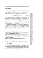
Fig. 6.1. Projection Theorem

We may extend all the above consideration to infinite-dimensional Hilbert
spaces H, if we consider closed subspaces V of H. Here closed means with

respect to the convergence induced by the norm. More precisely, a subset U ⊂ H
is closed in H if it contains all the limit points of sequences in U . Observe that if
V has finite dimension k, it is automatically closed, since it is isomorphic to Rk
(or Ck ). Also, a closed subspace of a Hilbert space is a Hilbert space as well, with
respect to the inner product in H.
Unless stated explicitly, from now on we consider Hilbert spaces over R
(real Hilbert spaces), endowed with inner product (·, ·) and induced norm · .


318

6 Elements of Functional Analysis

Theorem 6.2. (Projection Theorem). Let V be a closed subspace of a Hilbert
space H. Then, for every x ∈ H, there exists a unique element PV x ∈ V such that
PV x − x = inf v − x .

(6.17)

v∈V

Moreover, the following properties hold:
1. PV x = x if and only if x ∈ V .
2. Let QV x = x − PV x. Then QV x ∈ V ⊥ and
x
Proof. Let

2

= PV x

2

+ QV x

2

.

d = inf v − x .
v∈V

By the definition of least upper bound, we may select a sequence {vm } ⊂ V , such
that vm − x → d as m → ∞. In fact, for every integer m ≥ 1 there exists vm ∈ V
such that
1
d ≤ vm − x < d + .
(6.18)
m
Letting m → ∞ in (6.18), we get vm − x → d.
We now show that {vm } is a Cauchy sequence. In fact, using the parallelogram
law for the vectors vk − x and vm − x, we obtain
vk + vm − 2x
Since

vk +vm
2

2

2

+ vk − vm

= 2 vk − x

2

+ 2 vm − x

2

.

(6.19)

∈ V , we may write
vk + vm − 2x

2

=4

vk + vm
−x
2

2

≥ 4d2

whence, from (6.19):
vk − vm

2

= 2 vk − x

2

+ 2 vm − x

2

− vk + vm − 2x

≤ 2 vk − x

2

+ 2 vm − x

2

− 4d2 .

2

Letting k, m → ∞, the right hand side goes to zero and therefore
vk − vm → 0

as well. This proves that {vm } is a Cauchy sequence.
Since H is complete, vm converges to an element w ∈ H which belongs to V ,
because V is closed. Using the norm continuity (Proposition 6.1) we deduce
vm − x → w − x = d
so that w realizes the minimum distance from x among the elements in V .


6.4 Projections and Bases

319

We have to prove the uniqueness of w. Suppose w
¯ ∈ V is another element such
that w¯ − x = d. The parallelogram law, applied to the vectors w − x and w¯ − x,
yields
2

w − w¯

= 2 w−x

2

+ 2 w¯ − x

2

−4

w+w

¯
−x
2

2

≤ 2d2 + 2d2 − 4d2 = 0
whence w = w.
¯
We have proved that there exists a unique element w = PV x ∈ V such that
x − PV x = d.
To prove 1, observe that, since V is closed, x ∈ V if and only if d = 0, which means
x = PV x.
To show 2, let QV x = x − PV x, v ∈ V e t ∈ R. Since PV x + tv ∈ V for every
t, we have:
d2 ≤ x − (PV x + tv)
= QV x

2

2

= QV x − tv

− 2t (QV x, v) + t2 v

= d2 − 2t (QV x, v) + t2 v

2

2

2

.

Erasing d2 and dividing by t > 0, we get
(QV x, v) ≤

t
v
2

2

which forces (QV x, v) ≤ 0; dividing by t < 0 we get
(QV x, v) ≥

t
v
2

2

which forces (QV x, v) ≥ 0. Thus (QV x, v) = 0 which means QV x ∈ V ⊥ and
implies that
x 2 = P V x + QV x 2 = P V x 2 + QV x 2 ,
concluding the proof.
The elements PV x, QV x are called orthogonal projections of x on V and
V ⊥ , respectively. The least upper bound in (6.17) is actually a minimum. Moreover

thanks to properties 1, 2, we say that H is direct sum of V and V ⊥ :
H = V ⊕ V ⊥.
Note that
V ⊥ = {0}

if and only if

V = H.


320

6 Elements of Functional Analysis

Remark 6.3. Another characterization of PV x is the following (see Problem 6.4):
u = PV x if and only if
1. u ∈ V
2. (x − u, v) = 0, ∀v ∈ V.
Remark 6.4. It is useful to point out that, even if V is not a closed subspace of H,
the subspace V ⊥ is always closed. In fact, if yn → y and {yn } ⊂ V ⊥ , we have, for
every x ∈ V ,
(y, x) = lim (yn , x) = 0
whence y ∈ V ⊥ .
Example 6.5. Let Ω ⊂ Rn be a set of finite measure. Consider in L2 (Ω) the
1−dimensional subspace V of constant functions (a basis is given by f ≡ 1, for
instance). Since it is finite-dimensional, V is closed in L2 (Ω) . Given f ∈ L2 (Ω),
to find the projection PV f, we solve the minimization problem
(f − λ)2 .

min

λ∈R

Ω

Since
(f − λ)2 =
Ω

we see that the minimizer is
λ=
Therefore
PV f =

1
|Ω|

f

f + λ2 |Ω| ,

f 2 − 2λ
Ω

Ω

1
|Ω|

f.
Ω

QV f = f −

and

Ω

1
|Ω|

f.
Ω

Thus, the subspace V ⊥ is given by the functions g ∈ L2 (Ω) with zero mean value.
In fact these functions are orthogonal to f ≡ 1:
(g, 1)0 =

g = 0.
Ω

6.4.2 Bases
A Hilbert space is said to be separable when there exists a countable dense subset
of H. An orthonormal basis in a separable Hilbert space H is sequence {wk }k≥1 ⊂
H such that4
(wk , wj ) = δ kj
k, j ≥ 1, ...
k≥1
wk = 1
4

δjk is the Kronecker symbol.


6.4 Projections and Bases

321

and every x ∈ H may be expanded in the form
∞

x=

(x, wk ) wk .

(6.20)

k=1

The series (6.20) is called generalized Fourier series and the numbers ck =
(x, wk ) are the Fourier coefficients of x with respect to the basis {wk }. Moreover
(Pythagoras again!):
x

2

∞

2

=

(x, wk ) .
k=1

Given an orthonormal basis {wk }k≥1 , the projection of x ∈ H on the subspace V
spanned by, say, w1 , ..., wN is given by
N

PV x =

(x, wk ) wk .
k=1

An example of separable Hilbert space is L2 (Ω), Ω ⊆ Rn . In particular, the set of
functions
cos x sin x cos 2x sin 2x
1
cos mx sin mx
√ , √ , √ , √ , √ , ..., √
, √ , ...
π
π
π
π
π
π
2π
constitutes an orthonormal basis in L2 (0, 2π) (see Appendix A).
It turns out that:
Proposition 6.2. Every separable Hilbert space H admits an orthonormal basis.

Proof (sketch). Let {zk }k≥1 be dense in H. Disregarding, if necessary, those
elements which are spanned by other elements in the sequence, we may assume
that {zk }k≥1 constitutes an independent set, i.e. every finite subset of {zk }k≥1 is
composed by independent elements.
Then, an orthonormal basis {wk }k≥1 is obtained by applying to {zk }k≥1 the
following so called Gram-Schmidt process. First, construct by induction a sequence
{w}
˜ k≥1 as follows. Let w
˜ 1 = z1 . Once w
˜ k−1 is known, we construct w˜k by subtracting from zk its components with respect to w˜1 , ..., w
˜ k−1:
w
˜k = zk −

˜ k−1)
(zk , w
w
˜k−1

2

w
˜k−1 − · · · −

˜1)
(zk , w
w˜1

2

w˜1 .

In this way, w˜k is orthogonal to w
˜1 , ..., w
˜ k−1. Finally, set wk = w˜k / w
˜ k−1 . Since
{zk }k≥1 is dense in H, then {wk }k≥1 is dense in H as well. Thus {wk }k≥1 is an
orthonormal basis.
In the applications, orthonormal bases arise from solving particular boundary
value problems, often in relation to the separation of variables method. Typical
examples come form the vibrations of a non homogeneous string or from diffusion


322

6 Elements of Functional Analysis

in a rod with non constant thermal properties cv , ρ, κ. The first example leads to
the wave equation
ρ (x) utt − τ uxx = 0.
Separating variables (u(x, t) = v (x) z (t)), we find for the spatial factor the equation
τ v + λρv = 0.
In the second example we are led to
(κv ) + λcv ρv = 0.
These equations are particular cases of a general class of ordinary differential
equations of the form
(6.21)
(pu ) + qu + λwu = 0
called Sturm-Liouville equations. Usually one looks for solutions of (6.21) in an
interval (a, b), −∞ ≤ a < b ≤ +∞, satisfying suitable conditions at the end

points. The natural assumptions on p and q are p = 0 in (a, b) and p, q, p−1 locally
integrable in (a, b). The function w plays the role of a weight function, continuous
in [a, b] and positive in (a, b) .
In general, the resulting boundary value problem has non trivial solutions only
for particular values of λ, called eigenvalues. The corresponding solutions are called
eigenfunctions and it turns out that, when suitably normalized, they constitute an
orthonormal basis in the Hilbert space L2w (a, b), the set of Lebesgue measurable
functions in (a, b) such that
u

b

2
L2w

=

u2 (x) w (x) dx < ∞,

a

endowed with the inner product
b

(u, v)L2 =
w

u (x) v (x) w (x) dx.
a

We list below some examples5 .
• Consider the problem
1 − x2 u − xu + λu = 0
u (−1) < ∞,

in (−1, 1)

u (1) < ∞.

The differential equation is known as Chebyshev’s equation and may be written in
the form (6.21):
((1 − x2 )1/2 u ) + λ 1 − x2
5

For the proofs, see Courant-Hilbert, vol. I, 1953.

−1/2

u=0


6.4 Projections and Bases

323

−1/2

which shows the proper weight function w (x) = 1 − x2
. The eigenvalues
are λn = n2 , n = 0, 1, 2, .... The corresponding eigenfunctions are the Chebyshev

polynomials Tn , recursively defined by T0 (x) = 1, T1 (x) = x and
Tn+1 = 2xTn − Tn−1

(n > 1) .

For instance:
T2 (x) = 2x2 − 1, T3 (x) = 4x3 − 3x, T4 (x) = 8x4 − 8x2 − 1.
The normalized polynomials 1/πT0 ,
orthonormal basis in L2w (−1, 1).
• Consider the problem6
1 − x2 u

2/πT1 , ...,

+ λu = 0

2/πTn , ... constitute an

in (−1, 1)

with weighted Neumann conditions
1 − x2 u (x) → 0

as x → ±1.

The differential equation is known as Legendre’s equation. The eigenvalues are
λn = n (n + 1), n = 0, 1, 2, ... The corresponding eigenfunctions are the Legendre
polynomials, defined by L0 (x) = 1, L1 (x) = x,
(n + 1) Ln+1 = (2n + 1)xLn − nLn−1

(n > 1)

or by Rodrigues’ formula
Ln (x) =

1 dn
x2 − 1
2n n! dxn

n

(n ≥ 0) .

For instance, L2 (x) = (3x2 − 1)/2, L3 (x) = (5x3 − 3x)/2. The normalized polynomials
2n + 1
Ln
2
constitute an orthonormal basis in L2 (−1, 1) (here w (x) ≡ 1). Every function
f ∈ L2 (−1, 1) has an expansion
∞

f (x) =

fn Ln (x)
n=0

1

f (x) Ln (x) dx, with convergence in L2 (−1, 1).
where fn = 2n+1

2
−1
• Consider the problem
u − 2xu + 2λu = 0
e−x
6

See also Problem 8.5.

2

/2

u (x) → 0

in (−∞, +∞)
as x → ±∞.


324

6 Elements of Functional Analysis

The differential equation is known as Hermite’s equation (see Problem 6.6) and
may be written in the form (6.21):
2

2

(e−x u ) + 2λe−x u = 0

2

which shows the proper weight function w (x) = e−x . The eigenvalues are λn =
n, n = 0, 1, 2, .... The corresponding eigenfunctions are the Hermite polynomials
defined by Rodrigues’ formula
n

Hn (x) = (−1) ex

2

dn −x2
e
dxn

(n ≥ 0) .

For instance
H0 (x) = 1, H1 (x) = 2x, H2 (x) = 4x2 − 2, H3 (x) = 8x3 − 12x.
−1/2

Hn constitute an orthonormal basis
The normalized polynomials π −1/4 (2n n!)
2
in L2w (R), with w (x) = e−x . Every f ∈ L2w (R) has an expansion
∞

f (x) =

fn Hn (x)

n=0

where fn = [π 1/2 2n n!]−1

2

f (x) Hn (x) e−x dx, with convergence in L2w (R).

R

• After separating variables in the model for the vibration of a circular membrane the following parametric Bessel equation of order p arises (see Problem 6.8):
x2 u + xu + λx2 − p2 u = 0

x ∈ (0, a)

(6.22)

where p ≥ 0, λ ≥ 0, with the boundary conditions
u (0) finite,

u (a) = 0.

(6.23)

Equation (6.22) may be written in Sturm-Liouville form as
(xu ) + λx −

p2
x

u=0

which shows the proper weight function w (x) = x. The simple rescaling z =
reduces (6.22) to the Bessel equation of order p
z2

d2 u
du
+z
+ z 2 − p2 u = 0
dz 2
dz

√
λx

(6.24)

where the dependence on the parameter λ is removed. The only bounded solutions
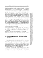
of (6.24) are the Bessel functions of first kind and order p, given by
∞

Jp (z) =
k=0

k

(−1)
Γ (k + 1) Γ (k + p + 1)

z
2

p+2k


6.4 Projections and Bases

325

Fig. 6.2. Graphs of J0 ,J1 and J2

where

∞

Γ (s) =

e−t ts−1 dt

(6.25)

0

is the Euler Γ − function. In particular, if p = n ≥ 0, integer:
∞

k

Jn (z) =

k=0

z
(−1)
k! (k + n)! 2

n+2k

.

For every p, there exists an infinite, increasing sequence {αpj }j≥1 of positive zeroes
of Jp :
Jp (αpj ) = 0

(j = 1, 2, ...).

αpj 2
Then, the eigenvalues of problem (6.22), (6.23) are given by λpj =
, with
a
αpj
corresponding eigenfunctions upj (x) = Jp
x . The normalized eigenfunctions
a
√
αpj
2
Jp
x
aJp+1 (αpj )

a
constitute an orthonormal basis in L2w (0, a), with w (x) = x. Every function f ∈
L2w (0, a) has an expansion in Fourier-Bessel series
∞

fj Jp

f (x) =
j=1

where
fj =
convergent in L2w (0, a).

a

2
2
a2 Jp+1
(αpj )

αpj
x ,
a

xf (x) Jp
0

αpj
x dx,

a


326

6 Elements of Functional Analysis

6.5 Linear Operators and Duality
6.5.1 Linear operators
Let H1 and H2 be Hilbert spaces. A linear operator from H1 into H2 is a
function
L : H1 → H2
such that7 , ∀α, β ∈ R and ∀x, y ∈ H1
L(αx + βy) = αLx + βLy.
For every linear operator we define its Kernel, N (L) and Range, R (L), as follows:
Definition 6.3. The kernel of L, is the pre-image of the null vector in H2 :
N (L) = {x ∈ H1 : Lx = 0} .
The range of L is the set of all outputs from points in H1 :
R (L) = {y ∈ H2 : ∃x ∈ H1 , Lx = y} .
N (L) and R (L) are linear subspaces of H1 and H2 , respectively.
Our main objects will be linear bounded operators.
Definition 6.4. A linear operator L : H1 → H2 is bounded if there exists a
number C such that
Lx

H2

≤C x

H1

∀x ∈ H1 .

,

(6.26)

The number C controls the expansion rate operated by L on the elements of
H1 . In particular, if C < 1, L contracts the sizes of the vectors in H1 .
If x = 0, using the linearity of L, we may write (6.26) in the form
L

x
x H1

≤C
H2

which is equivalent to
sup
x

since x/ x

H1

H1 =1

Lx

H2

= K < ∞,

(6.27)

is a unit vector in H1 . Clearly K ≤ C.

Proposition 6.3. A linear operator L : H1 → H2 is bounded if and only if it is
continuous.
7

Notation: if L is linear, when no confusion arises, we may write Lx instead of L (x).