Partial Differential Equations part 2

834
Chapter 19. Partial Differential Equations
Sample page from NUMERICAL RECIPES IN C: THE ART OF SCIENTIFIC COMPUTING (ISBN 0-521-43108-5)
Copyright (C) 1988-1992 by Cambridge University Press.Programs Copyright (C) 1988-1992 by Numerical Recipes Software.
Permission is granted for internet users to make one paper copy for their own personal use. Further reproduction, or any copying of machine-
readable files (including this one) to any servercomputer, is strictly prohibited. To order Numerical Recipes books,diskettes, or CDROMs
visit website or call 1-800-872-7423 (North America only),or send email to (outside North America).
engineering; these methods allow considerable freedom in putting computational
elements whereyou want them, importantwhendealing withhighlyirregular geome-
tries. Spectral methods
[13-15]
are preferred for very regular geometries and smooth
functions; they converge more rapidly than finite-difference methods (cf. §19.4), but
they do not work well for problems with discontinuities.
CITED REFERENCES AND FURTHER READING:
Ames, W.F. 1977,
Numerical Methods for Partial Differential Equations
, 2nd ed. (New York:
Academic Press). [1]
Richtmyer, R.D., and Morton, K.W. 1967,
Difference Methods for Initial Value Problems
, 2nd ed.
(New York: Wiley-Interscience). [2]
Roache, P.J. 1976,
Computational Fluid Dynamics
(Albuquerque: Hermosa). [3]
Mitchell, A.R., and Griffiths, D.F. 1980,
The Finite Difference Method in Partial Differential Equa-
tions
(New York: Wiley) [includes discussion of finite element methods]. [4]
Dorr, F.W. 1970,

SIAM Review
, vol. 12, pp. 248–263. [5]
Meijerink, J.A., and van der Vorst, H.A. 1977,
Mathematics of Computation
, vol. 31, pp. 148–
162. [6]
van der Vorst, H.A. 1981,
Journal of Computational Physics
, vol. 44, pp. 1–19 [review of sparse
iterative methods]. [7]
Kershaw, D.S. 1970,
Journal of Computational Physics
, vol. 26, pp. 43–65. [8]
Stone, H.J. 1968,
SIAM Journal on Numerical Analysis
, vol. 5, pp. 530–558. [9]
Jesshope, C.R. 1979,
Computer Physics Communications
, vol. 17, pp. 383–391. [10]
Strang, G., and Fix, G. 1973,
An Analysis of the Finite Element Method
(Englewood Cliffs, NJ:
Prentice-Hall). [11]
Burnett, D.S. 1987,
Finite Element Analysis: From Concepts to Applications
(Reading, MA:
Addison-Wesley). [12]
Gottlieb, D. and Orszag, S.A. 1977,
Numerical Analysis of Spectral Methods: Theory and Ap-
plications

(Philadelphia: S.I.A.M.). [13]
Canuto, C., Hussaini, M.Y., Quarteroni, A., and Zang, T.A. 1988,
Spectral Methods in Fluid
Dynamics
(New York: Springer-Verlag). [14]
Boyd, J.P. 1989,
Chebyshev and Fourier Spectral Methods
(New York: Springer-Verlag). [15]
19.1 Flux-Conservative Initial Value Problems
A large class of initial value (time-evolution) PDEs in one space dimension can
be cast into the form of a flux-conservative equation,
∂u
∂t
= −
∂F(u)
∂x
(19.1.1)
where u and F are vectors, and where (in some cases) F may depend not only on u
but also on spatial derivatives of u. The vector F is called the conserved flux.
For example, the prototypical hyperbolic equation, the one-dimensional wave
equation with constant velocity of propagation v
∂
2
u
∂t
2
= v
2
∂
2

u
∂x
2
(19.1.2)
19.1 Flux-Conservative Initial Value Problems
835
Sample page from NUMERICAL RECIPES IN C: THE ART OF SCIENTIFIC COMPUTING (ISBN 0-521-43108-5)
Copyright (C) 1988-1992 by Cambridge University Press.Programs Copyright (C) 1988-1992 by Numerical Recipes Software.
Permission is granted for internet users to make one paper copy for their own personal use. Further reproduction, or any copying of machine-
readable files (including this one) to any servercomputer, is strictly prohibited. To order Numerical Recipes books,diskettes, or CDROMs
visit website or call 1-800-872-7423 (North America only),or send email to (outside North America).
can be rewritten as a set of two first-order equations
∂r
∂t
= v
∂s
∂x
∂s
∂t
= v
∂r
∂x
(19.1.3)
where
r ≡ v
∂u
∂x
s ≡
∂u
∂t

(19.1.4)
In this case r and s become the two components of u, and the flux is given by
the linear matrix relation
F(u)=

0 −v
−v 0

·u (19.1.5)
(The physicist-reader may recognize equations (19.1.3) as analogous to Maxwell’s
equations for one-dimensional propagation of electromagnetic waves.)
We will consider, in this section, a prototypical example of the general flux-
conservative equation (19.1.1), namely the equation for a scalar u,
∂u
∂t
= −v
∂u
∂x
(19.1.6)
with v a constant. As it happens, we already know analytically that the general
solution of this equation is a wave propagating in the positive x-direction,
u = f(x − vt)(19.1.7)
where f is an arbitrary function. However, the numerical strategies that we develop
will be equally applicable to the more general equations represented by (19.1.1). In
some contexts, equation (19.1.6) iscalled an advective equation, because the quantity
u is transported by a “fluid flow” with a velocity v.
How do we go about finite differencing equation (19.1.6) (or, analogously,
19.1.1)? The straightforward approach is to choose equally spaced points along both
the t-andx-axes. Thus denote
x

j
= x
0
+ j∆x, j =0,1,...,J
t
n
=t
0
+n∆t, n =0,1,...,N
(19.1.8)
Let u
n
j
denote u(t
n
,x
j
). We have several choices for representing the time
derivative term. The obvious way is to set
∂u
∂t




j,n
=
u
n+1
j

− u
n
j
∆t
+ O(∆t)(19.1.9)
This is called forward Euler differencing (cf. equation 16.1.1). While forward Euler
is only first-order accurate in ∆t, it has the advantage that one is able to calculate
836
Chapter 19. Partial Differential Equations
Sample page from NUMERICAL RECIPES IN C: THE ART OF SCIENTIFIC COMPUTING (ISBN 0-521-43108-5)
Copyright (C) 1988-1992 by Cambridge University Press.Programs Copyright (C) 1988-1992 by Numerical Recipes Software.
Permission is granted for internet users to make one paper copy for their own personal use. Further reproduction, or any copying of machine-
readable files (including this one) to any servercomputer, is strictly prohibited. To order Numerical Recipes books,diskettes, or CDROMs
visit website or call 1-800-872-7423 (North America only),or send email to (outside North America).
t or n
x or j
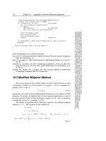
FTCS
Figure 19.1.1. Representation of the Forward Time CenteredSpace (FTCS) differencing scheme. In this
and subsequentfigures, the open circle is the new point at which the solution is desired; filled circles are
known points whose function values are used in calculating the new point; the solid lines connect points
that are used to calculate spatial derivatives; the dashedlines connect pointsthat are used to calculate time
derivatives. The FTCS scheme is generallyunstable for hyperbolicproblems and cannotusually be used.
quantities at timestep n +1in terms of only quantities known at timestep n.Forthe
space derivative, we can use a second-order representation still using only quantities
known at timestep n:
∂u
∂x





j,n
=
u
n
j+1
− u
n
j −1
2∆x
+ O(∆x
2
)(19.1.10)
The resulting finite-difference approximation to equation (19.1.6) is called the FTCS
representation (Forward Time Centered Space),
u
n+1
j
− u
n
j
∆t
= −v

u
n
j+1
− u
n
j −1

2∆x

(19.1.11)
which can easily be rearranged to be a formula for u
n+1
j
in terms of the other
quantities. The FTCS scheme is illustrated in Figure 19.1.1. It’s a fine example of
an algorithm that is easy to derive, takes little storage, and executes quickly. Too
bad it doesn’t work! (See below.)
The FTCS representation is an explicit scheme. This means that u
n+1
j
for each
j can be calculated explicitly from the quantities that are already known. Later we
shall meet implicit schemes, which require us to solve implicit equations coupling
the u
n+1
j
for various j. (Explicit and implicit methods for ordinary differential
equations were discussed in §16.6.) The FTCS algorithm is also an example of
a single-level scheme, since only values at time level n have to be stored to find
values at time level n +1.
von Neumann Stability Analysis
Unfortunately, equation (19.1.11) is of very limited usefulness. It is an unstable
method, which can be used only (if at all) to study waves for a short fraction of one
oscillation period. To find alternative methods with more general applicability, we
must introduce the von Neumann stability analysis.
The von Neumann analysis is local: We imagine that the coefficients of the
difference equations are so slowly varying as to be considered constant in space

and time. In that case, the independent solutions, or eigenmodes, of the difference
equations are all of the form
u
n
j
= ξ
n
e
ikj∆x
(19.1.12)
19.1 Flux-Conservative Initial Value Problems
837
Sample page from NUMERICAL RECIPES IN C: THE ART OF SCIENTIFIC COMPUTING (ISBN 0-521-43108-5)
Copyright (C) 1988-1992 by Cambridge University Press.Programs Copyright (C) 1988-1992 by Numerical Recipes Software.
Permission is granted for internet users to make one paper copy for their own personal use. Further reproduction, or any copying of machine-
readable files (including this one) to any servercomputer, is strictly prohibited. To order Numerical Recipes books,diskettes, or CDROMs
visit website or call 1-800-872-7423 (North America only),or send email to (outside North America).
t or n
x or j
Lax
Figure 19.1.2. Representation of the Lax differencing scheme, as in the previous figure. The stability
criterion for this scheme is the Courant condition.
where k is a real spatial wave number (which can have any value) and ξ = ξ(k) is
a complex number that depends on k. The key fact is that the time dependence of
a single eigenmode is nothing more than successive integer powers of the complex
number ξ. Therefore, the difference equations are unstable (have exponentially
growing modes) if |ξ(k)| > 1 for some k. The number ξ is called the amplification
factor at a given wave number k.
To find ξ (k ), we simply substitute (19.1.12) back into (19.1.11). Dividing
by ξ

n
,weget
ξ(k)=1−i
v∆t
∆x
sin k∆x (19.1.13)
whose modulus is > 1 for all k; so the FTCS scheme is unconditionally unstable.
If the velocity v were a function of t and x, then we would write v
n
j
in equation
(19.1.11). In the von Neumann stability analysis we would still treat v as a constant,
theideabeingthatforvslowly varying the analysis is local. In fact, even in the
case of strictly constant v, the von Neumann analysis does not rigorously treat the
end effects at j =0and j = N.
More generally, if the equation’s right-hand side were nonlinear in u,thena
von Neumann analysis would linearize by writing u = u
0
+ δu, expanding to linear
order in δu. Assuming that the u
0
quantities already satisfy the difference equation
exactly, the analysis would look for an unstable eigenmode of δu.
Despite its lack of rigor, the von Neumann method generally gives valid
answers and is much easier to apply than more careful methods. We accordingly
adopt it exclusively. (See, for example,
[1]
for a discussion of other methods of
stability analysis.)
Lax Method

The instabilityin the FTCS method can be cured by a simplechange due to Lax.
One replaces the term u
n
j
in the time derivative term by its average (Figure 19.1.2):
u
n
j
→
1
2

u
n
j+1
+ u
n
j −1

(19.1.14)
This turns (19.1.11) into
u
n+1
j
=
1
2

u
n

j+1
+ u
n
j −1

−
v∆t
2∆x

u
n
j+1
− u
n
j −1

(19.1.15)
838
Chapter 19. Partial Differential Equations
Sample page from NUMERICAL RECIPES IN C: THE ART OF SCIENTIFIC COMPUTING (ISBN 0-521-43108-5)
Copyright (C) 1988-1992 by Cambridge University Press.Programs Copyright (C) 1988-1992 by Numerical Recipes Software.
Permission is granted for internet users to make one paper copy for their own personal use. Further reproduction, or any copying of machine-
readable files (including this one) to any servercomputer, is strictly prohibited. To order Numerical Recipes books,diskettes, or CDROMs
visit website or call 1-800-872-7423 (North America only),or send email to (outside North America).
t or n
∆t
x or j
∆t
∆x∆x
unstablestable

(a) (b)
Figure 19.1.3. Courant condition for stability of a differencing scheme. The solution of a hyperbolic
problem at a point depends on information within some domain of dependency to the past, shown here
shaded. The differencing scheme (19.1.15) has its own domain of dependency determined by the choice
of points on one time slice (shown as connected solid dots) whose values are used in determining a new
point (shown connected by dashed lines). A differencing scheme is Courant stable if the differencing
domain of dependency is larger than that of the PDEs, as in (a), and unstable if the relationship is the
reverse, as in (b). For more complicated differencing schemes, the domain of dependency might not be
determined simply by the outermost points.
Substituting equation (19.1.12), we find for the amplification factor
ξ =cosk∆x−i
v∆t
∆x
sin k∆x (19.1.16)
The stability condition |ξ|
2
≤ 1 leads to the requirement
|v|∆t
∆x
≤ 1(19.1.17)
This is the famous Courant-Friedrichs-Lewy stability criterion, often
called simply the Courant condition. Intuitively, the stability condition can be
understood as follows (Figure 19.1.3): The quantity u
n+1
j
in equation (19.1.15) is
computed from information at points j − 1 and j +1at time n.Inotherwords,
x
j−1
and x

j+1
arethe boundariesof the spatialregionthatisallowed tocommunicate
information to u
n+1
j
. Now recall that in the continuum wave equation, information
actually propagates with a maximum velocity v. If the point u
n+1
j
is outside of
the shaded region in Figure 19.1.3, then it requires information from points more
distant than the differencing scheme allows. Lack of that information gives rise to
an instability. Therefore, ∆t cannot be made too large.
The surprising result, that the simple replacement (19.1.14) stabilizes the FTCS
scheme, is our first encounter with the fact that differencing PDEs is an art as much
as a science. To see if we can demystify the art somewhat, let us compare the
FTCS and Lax schemes by rewriting equation (19.1.15) so that it is in the form of
equation (19.1.11) with a remainder term:
u
n+1
j
− u
n
j
∆t
= −v

u
n
j+1

− u
n
j −1
2∆x

+
1
2

u
n
j+1
− 2u
n
j
+ u
n
j −1
∆t

(19.1.18)
But this is exactly the FTCS representation of the equation
∂u
∂t
= −v
∂u
∂x
+
(∆x)
2

2∆t
∇
2
u (19.1.19)