Partial Differential Equations part 1

Sample page from NUMERICAL RECIPES IN C: THE ART OF SCIENTIFIC COMPUTING (ISBN 0-521-43108-5)
Copyright (C) 1988-1992 by Cambridge University Press.Programs Copyright (C) 1988-1992 by Numerical Recipes Software.
Permission is granted for internet users to make one paper copy for their own personal use. Further reproduction, or any copying of machine-
readable files (including this one) to any servercomputer, is strictly prohibited. To order Numerical Recipes books,diskettes, or CDROMs
visit website or call 1-800-872-7423 (North America only),or send email to (outside North America).
Chapter 19. Partial Differential
Equations
19.0 Introduction
The numerical treatment of partial differential equations is, by itself, a vast
subject. Partial differential equations are at the heart of many, if not most,
computer analyses or simulations of continuous physical systems, such as fluids,
electromagnetic fields, the human body, and so on. The intent of this chapter is to
givethe briefest possibleuseful introduction. Ideally, therewouldbe an entiresecond
volume of Numerical Recipes dealing with partial differential equations alone. (The
references
[1-4]
provide, of course, available alternatives.)
In most mathematics books, partial differential equations (PDEs) are classified
into the three categories, hyperbolic, parabolic, and elliptic, on the basis of their
characteristics, or curves of information propagation. The prototypical example of
a hyperbolic equation is the one-dimensional wave equation
∂
2
u
∂t
2
= v
2
∂
2
u

∂x
2
(19.0.1)
where v = constant is the velocity of wave propagation. The prototypicalparabolic
equation is the diffusion equation
∂u
∂t
=
∂
∂x

D
∂u
∂x

(19.0.2)
where D is the diffusion coefficient. The prototypical elliptic equation is the
Poisson equation
∂
2
u
∂x
2
+
∂
2
u
∂y
2
= ρ(x, y)(19.0.3)

where the source term ρ is given. If the source term is equal to zero, the equation
is Laplace’s equation.
From a computational point of view, the classification into these three canonical
types is not very meaningful — or at least not as important as some other essential
distinctions. Equations (19.0.1) and (19.0.2) both define initial value or Cauchy
problems: If information on u (perhaps including time derivative information) is
827
828
Chapter 19. Partial Differential Equations
Sample page from NUMERICAL RECIPES IN C: THE ART OF SCIENTIFIC COMPUTING (ISBN 0-521-43108-5)
Copyright (C) 1988-1992 by Cambridge University Press.Programs Copyright (C) 1988-1992 by Numerical Recipes Software.
Permission is granted for internet users to make one paper copy for their own personal use. Further reproduction, or any copying of machine-
readable files (including this one) to any servercomputer, is strictly prohibited. To order Numerical Recipes books,diskettes, or CDROMs
visit website or call 1-800-872-7423 (North America only),or send email to (outside North America).
.
.
.
.
.
.
.
.
.
.
.
.
.
.
.
.

.
.
.
.
.
boundary
conditions
initial values
(a)
boundary
values
(b)
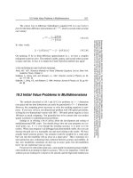
Figure 19.0.1. Initial value problem (a) and boundary value problem (b) are contrasted. In (a) initial
values are given on one “time slice,” and it is desired to advance the solution in time, computing
successive rows of open dots in the direction shown by the arrows. Boundary conditions at the left and
right edges of each row (⊗) must also be supplied, but only one row at a time. Only one, or a few,
previous rows need be maintained in memory. In (b), boundary values are specified around the edge of
a grid, and an iterative process is employed to find the values of all the internal points (open circles).
All grid points must be maintained in memory.
given at some initial time t
0
for all x, then the equations describe how u(x, t)
propagates itself forward in time. In other words, equations (19.0.1) and (19.0.2)
describe time evolution. The goal of a numerical code should be to track that time
evolution with some desired accuracy.
By contrast, equation (19.0.3) directs us to find a single “static” function u(x, y)
which satisfies the equation within some (x, y) region of interest, and which — one
must also specify — has some desired behavior on the boundary of the region of
interest. These problems are called boundary value problems. In general it is not
19.0 Introduction

829
Sample page from NUMERICAL RECIPES IN C: THE ART OF SCIENTIFIC COMPUTING (ISBN 0-521-43108-5)
Copyright (C) 1988-1992 by Cambridge University Press.Programs Copyright (C) 1988-1992 by Numerical Recipes Software.
Permission is granted for internet users to make one paper copy for their own personal use. Further reproduction, or any copying of machine-
readable files (including this one) to any servercomputer, is strictly prohibited. To order Numerical Recipes books,diskettes, or CDROMs
visit website or call 1-800-872-7423 (North America only),or send email to (outside North America).
possible stably to just “integrate in from the boundary” in the same sense that an
initial value problem can be “integrated forward in time.” Therefore, the goal of a
numerical code is somehow to converge on the correct solution everywhere at once.
This, then, is the most important classification from a computational point
of view: Is the problem at hand an initial value (time evolution) problem? or
is it a boundary value (static solution) problem? Figure 19.0.1 emphasizes the
distinction. Notice that while the italicized terminology is standard, the terminology
in parentheses is a much better description of the dichotomy from a computational
perspective. The subclassification of initial value problems into parabolic and
hyperbolic is much less important because (i) many actual problems are of a mixed
type, and (ii) as we will see, most hyperbolic problems get parabolic pieces mixed
into them by the time one is discussing practical computational schemes.
Initial Value Problems
An initial value problem is defined by answers to the following questions:
• What are the dependent variables to be propagated forward in time?
• What is the evolution equation for each variable? Usually the evolution
equations will all be coupled, with more than one dependent variable
appearing on the right-hand side of each equation.
• What is the highest time derivative that occurs in each variable’s evolution
equation? If possible, this time derivative should be put alone on the
equation’s left-hand side. Not only the value of a variable, but also the
value of all its time derivatives — up to the highest one — must be
specified to define the evolution.
• What special equations (boundary conditions) govern the evolutionin time

of points on the boundary of the spatial region of interest? Examples:
Dirichletconditionsspecify the values of the boundarypoints as a function
of time; Neumann conditionsspecify the values of the normal gradients on
the boundary; outgoing-wave boundary conditions are just what they say.
Sections 19.1–19.3 of this chapter deal with initial value problems of several
different forms. We make no pretence of completeness, but rather hope to convey a
certain amount of generalizable information through a few carefully chosen model
examples. These examples will illustrate an important point: One’s principal
computational concern must be the stability of the algorithm. Many reasonable-
looking algorithmsfor initial value problems just don’t work — they are numerically
unstable.
Boundary Value Problems
The questions that define a boundary value problem are:
• What are the variables?
• What equations are satisfied in the interior of the region of interest?
• What equations are satisfied by points on the boundary of the region of
interest? (Here Dirichlet and Neumann conditions are possible choices for
ellipticsecond-order equations,but morecomplicated boundaryconditions
can also be encountered.)
830
Chapter 19. Partial Differential Equations
Sample page from NUMERICAL RECIPES IN C: THE ART OF SCIENTIFIC COMPUTING (ISBN 0-521-43108-5)
Copyright (C) 1988-1992 by Cambridge University Press.Programs Copyright (C) 1988-1992 by Numerical Recipes Software.
Permission is granted for internet users to make one paper copy for their own personal use. Further reproduction, or any copying of machine-
readable files (including this one) to any servercomputer, is strictly prohibited. To order Numerical Recipes books,diskettes, or CDROMs
visit website or call 1-800-872-7423 (North America only),or send email to (outside North America).
In contrast to initial value problems, stability is relatively easy to achieve
for boundary value problems. Thus, the efficiency of the algorithms, both in
computational load and storage requirements, becomes the principal concern.
Because all the conditions on a boundary value problem must be satisfied

“simultaneously,” these problems usually boil down, at least conceptually, to the
solutionof large numbers of simultaneous algebraic equations. When such equations
are nonlinear, they are usually solved by linearization and iteration; so without much
loss of generality we can view the problem as being the solution of special, large
linear sets of equations.
As an example, one which we will refer to in §§19.4–19.6 as our “model
problem,” let us consider the solution of equation (19.0.3) by the finite-difference
method. We represent the function u(x, y) by its values at the discrete set of points
x
j
= x
0
+ j∆,j=0,1, ..., J
y
l
= y
0
+ l∆,l=0,1, ..., L
(19.0.4)
where ∆ is the grid spacing. From now on, we will write u
j,l
for u(x
j
,y
l
),and
ρ
j,l
for ρ(x
j

,y
l
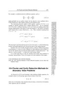
). For (19.0.3) we substitute a finite-difference representation (see
Figure 19.0.2),
u
j+1,l
− 2u
j,l
+ u
j−1,l
∆
2
+
u
j,l+1
− 2u
j,l
+ u
j,l−1
∆
2
= ρ
j,l
(19.0.5)
or equivalently
u
j+1,l
+ u
j−1,l
+ u

j,l+1
+ u
j,l−1
− 4u
j,l
=∆
2
ρ
j,l
(19.0.6)
To write this system of linear equations in matrix form we need to make a
vector out of u. Let us number the two dimensions of grid points in a single
one-dimensional sequence by defining
i ≡ j(L +1)+l for j =0,1, ..., J, l =0,1, ..., L (19.0.7)
In other words, i increases most rapidly along the columns representing y values.
Equation (19.0.6) now becomes
u
i+L+1
+ u
i−(L+1)
+ u
i+1
+ u
i−1
− 4u
i
=∆
2
ρ
i

(19.0.8)
This equation holds only at the interior points j =1,2, ..., J − 1; l =1,2, ...,
L − 1.
The points where
j =0
j=J
l=0
l=L
[i.e., i =0, ..., L]
[i.e., i = J(L +1), ..., J(L +1)+L]
[i.e., i =0,L+1, ..., J(L +1)]
[i.e., i = L, L +1+L, ..., J(L +1)+L]
(19.0.9)
19.0 Introduction
831
Sample page from NUMERICAL RECIPES IN C: THE ART OF SCIENTIFIC COMPUTING (ISBN 0-521-43108-5)
Copyright (C) 1988-1992 by Cambridge University Press.Programs Copyright (C) 1988-1992 by Numerical Recipes Software.
Permission is granted for internet users to make one paper copy for their own personal use. Further reproduction, or any copying of machine-
readable files (including this one) to any servercomputer, is strictly prohibited. To order Numerical Recipes books,diskettes, or CDROMs
visit website or call 1-800-872-7423 (North America only),or send email to (outside North America).
y
L
∆
y
1
y
0
x
0
x

J
x
1
...
∆
A
B
Figure 19.0.2. Finite-difference representation of a second-order elliptic equation on a two-dimensional
grid. The secondderivatives at the point A are evaluated using the points to which A is shown connected.
The second derivatives at point B are evaluated using the connected points and also using “right-hand
side” boundary information, shown schematically as ⊗.
are boundary points where either u or its derivative has been specified. If we pull
all this “known” information over to the right-hand side of equation (19.0.8), then
the equation takes the form
A · u = b (19.0.10)
where A has the form shown in Figure 19.0.3. The matrix A is called “tridiagonal
with fringes.” A general linear second-order elliptic equation
a(x, y)
∂
2
u
∂x
2
+ b(x, y)
∂u
∂x
+ c(x, y)
∂
2
u

∂y
2
+ d(x, y)
∂u
∂y
+ e(x, y)
∂
2
u
∂x∂y
+ f(x, y)u = g(x, y)
(19.0.11)
will lead to a matrix of similar structure except that the nonzero entries will not
be constants.
As a rough classification, there are three different approaches to the solution
of equation (19.0.10), not all applicable in all cases: relaxation methods, “rapid”
methods (e.g., Fourier methods), and direct matrix methods.