Development of a ball balancing robot
Bạn đang xem bản rút gọn của tài liệu. Xem và tải ngay bản đầy đủ của tài liệu tại đây (5.95 MB, 65 trang )
ISSN 0280-5316
ISRN LUTFD2/TFRT--5897--SE
Development of a ball balancing robot
with omni wheels
Magnus Jonason Bjärenstam
Michael Lennartsson
Lund University
Department of Automatic Control
March 2012
Lund University
Department of Automatic Control
Box 118
SE-221 00 Lund Sweden
Document name
Author(s)
Supervisor
Magnus Jonason Bjärenstam
Michael Lennartsson
Anders Robertsson, Dept. of Automatic
Control, Lund University, Sweden
Rolf Johansson, Dept. of Automatic Control,
Lund University, Sweden (examiner)
MASTER THESIS
Date of issue
March 2012
Document Number
ISRN LUTFD2/TFRT--5897--SE
Sponsoring organization
Title and subtitle
Development of a ball-balancing robot with omni-wheels (Bollbalanserande robot med omnihjul)
Abstract
The main goal for this master thesis project was to create a robot balancing on a ball with the help of
omni wheels. The robot was developed from scratch. The work covered everything from mechanical
design, dynamic modeling, control design, sensor fusion, identifying parameters by experimentation
to implementation on a microcontroller. The robot has three omni wheels in a special configuration at
the bottom. The task to stabilize the robot is based on the simplified model of controlling a spherical
inverted pendulum in the xy-plane with state feedback control. The model has accelerations in the
bottom in the x- and y-directions as inputs. The controlled outputs are the angle and angular velocity
around the x- and y-axes and the position and speed along the same axes.The goal to stabilize the
robot in an upright position and keep it located around the starting point was successfully achieved.
Keywords
Classification system and/or index terms (if any)
Supplementary bibliographical information
ISSN and key title
ISBN
0280-5316
Language
Number of pages
English
1-63
Security classification
/>
Recipient’s notes
Acknowledgement
We would like to thank our supervisor Anders Robertsson who has been very
helpful and supporting all our ideas, Rolf Braun for his great assistance in
hardware issues and building (and repairing) the robot and Leif Andersson
for helping us with various computer problems.
Magnus & Michael
1
2
Contents
1 Introduction
2 Hardware
2.1 Mecanum wheel . . . . .
2.2 Omni wheels . . . . . .
2.3 Lego Mindstorms . . . .
2.4 Arduino Mega 2560 . . .
2.5 ArduIMU+ V3 . . . . .
2.6 Faulhaber MCDC 3006S
5
. . . . . . . . .
. . . . . . . . .
. . . . . . . . .
. . . . . . . . .
. . . . . . . . .
& 3257G012CR
.
.
.
.
.
.
.
.
.
.
.
.
.
.
.
.
.
.
.
.
.
.
.
.
.
.
.
.
.
.
.
.
.
.
.
.
.
.
.
.
.
.
.
.
.
.
.
.
.
.
.
.
.
.
.
.
.
.
.
.
.
.
.
.
.
.
.
.
.
.
.
.
6
6
6
8
9
9
10
3 Theoretical Background
3.1 State feedback control . . . . . . . . . . . . . . .
3.2 Linear Quadratic Optimal Control . . . . . . . .
3.3 Complementary filter . . . . . . . . . . . . . . . .
3.4 Kinematics . . . . . . . . . . . . . . . . . . . . .
3.4.1 Kinematics of omni and mecanum wheels
3.4.2 Kinematics of the Test Rig . . . . . . . .
3.4.3 Ball translation . . . . . . . . . . . . . . .
3.4.4 Robot translation . . . . . . . . . . . . . .
.
.
.
.
.
.
.
.
.
.
.
.
.
.
.
.
.
.
.
.
.
.
.
.
.
.
.
.
.
.
.
.
.
.
.
.
.
.
.
.
.
.
.
.
.
.
.
.
.
.
.
.
.
.
.
.
11
11
12
12
13
13
15
17
19
4 Methodology
4.1 Platforms . . . . . . . . . . . . . .
4.1.1 Omni wheel platform . . . .
4.1.2 Mecanum wheel platform .
4.1.3 Lego Mindstorms Platform
4.2 The Test Rig . . . . . . . . . . . .
4.2.1 Geometry and design . . . .
4.2.2 Verification . . . . . . . . .
4.3 The Robot . . . . . . . . . . . . .
4.3.1 Dynamics of the Robot . .
4.3.2 Dymola Model . . . . . . .
4.3.3 Robot design . . . . . . . .
4.3.4 Implementation . . . . . . .
.
.
.
.
.
.
.
.
.
.
.
.
.
.
.
.
.
.
.
.
.
.
.
.
.
.
.
.
.
.
.
.
.
.
.
.
.
.
.
.
.
.
.
.
.
.
.
.
.
.
.
.
.
.
.
.
.
.
.
.
.
.
.
.
.
.
.
.
.
.
.
.
.
.
.
.
.
.
.
.
.
.
.
.
22
22
22
23
26
27
28
28
29
29
30
32
32
3
.
.
.
.
.
.
.
.
.
.
.
.
.
.
.
.
.
.
.
.
.
.
.
.
.
.
.
.
.
.
.
.
.
.
.
.
.
.
.
.
.
.
.
.
.
.
.
.
.
.
.
.
.
.
.
.
.
.
.
.
.
.
.
.
.
.
.
.
.
.
.
.
.
.
.
.
.
.
.
.
.
.
.
.
.
.
.
.
.
.
.
.
.
.
.
.
5 Results
5.1 Lego Robot . . . . . . . . . .
5.2 Test Rig Kinematics . . . . .
5.3 The Robot . . . . . . . . . .
5.3.1 Linear Model . . . . .
5.3.2 Model Simulations . .
5.3.3 Complementary Filter
5.3.4 Robot Performance . .
.
.
.
.
.
.
.
.
.
.
.
.
.
.
.
.
.
.
.
.
.
.
.
.
.
.
.
.
.
.
.
.
.
.
.
.
.
.
.
.
.
.
.
.
.
.
.
.
.
.
.
.
.
.
.
.
.
.
.
.
.
.
.
.
.
.
.
.
.
.
.
.
.
.
.
.
.
.
.
.
.
.
.
.
.
.
.
.
.
.
.
.
.
.
.
.
.
.
.
.
.
.
.
.
.
.
.
.
.
.
.
.
.
.
.
.
.
.
.
.
.
.
.
.
.
.
37
37
37
38
38
39
40
40
6 Conclusion and Future Work
45
A Source-code
48
4
Chapter 1
Introduction
The goal of this Master Thesis was to build and stabilize a robot balancing on a ball, inspired by a Japanese project [1]. The authors’ background
is in mechatronical engineering and therefore this project was a suitable
challenge.
The robot consists of three omni wheels in a special configuration standing on a ball which gives it inverse pendulum dynamics. The robot is stabilized by rotating the wheels which makes it move in the xy-plane.
First the kinematics of omni wheels was investigated by studying different mounting configurations on platforms moving on the ground [2]. A Lego
robot was built to verify and visualize the kinematics and special properties
of omni wheels.
Then a model of an inverted pendulum was developed in parallel with the
kinematics of a ball actuated by three omni wheels. The inverted pendulum
model in the xy-plane was developed in Dymola and exported to Matlab to
perform state feedback controller design. The designed controller was then
imported back into Dymola for simulation and visualization.
The model of the inverted pendulum has eight states. The states are
angle, angular velocity, position, and velocity along the x- and y-axes. State
feedback requires measurements from all states. The angles are estimated
with sensor fusion done by a complementary filter combining gyroscope and
accelerometer readings. The velocities are obtained by using motor readings
and inverse kinematics which are integrated to get the positions.
The implementation was done on an Arduino microcontroller board.
5
Chapter 2
Hardware
In this chapter the hardware used and how it is setup is covered.
2.1
Mecanum wheel
The mecanum wheel, also called the Ilon wheel, was invented by the Swedish
inventor Bengt Ilon in 1973 when he worked at the Swedish company Mecanum
AB. The mecanum wheel is a conventional wheel with a series of rollers connected with an angle to the circumference. The axes of rotation for the
rollers are usually in 45 degree angle to the circumference of the mecanum
wheel, see Figure 2.1. This configuration of rollers enables the mecanum
wheel to move in both the rotational and the lateral direction of the wheel.
On a platform with two mecanum wheel pairs in parallel there are actually two versions of the mecanum wheel, one with the roller axis mounted
+45 degrees with respect to the wheels axis and the other with the roller axis
rotated -45 degrees to the wheel axis, see Figure 2.2. One of the mecanum
wheels in each pair has the positive angle and the other one has the negative.
If that was not the case all of the resultants for the four mecanum wheels
would have been parallel and the ability to move in any direction had been
lost.
The mecanum wheels are used on platforms where movement in tight
and narrow spaces is crucial for example on forklifts inside warehouses [3].
2.2
Omni wheels
Omni-directional wheels also have rollers connected to the circumference like
the mecanum wheel, see Figure 2.3. The difference between the mecanum
wheel and the omni wheel is that the axes of rotation for the rollers is parallel
to the circumference of the wheel instead of 45 degrees as for the mecanum
wheel. This design with the rollers enables the omni wheel to move freely in
two directions. It can either roll around the wheel axis like a regular wheel
6
Figure 2.1: Mecanum wheel.
Figure 2.2: The two different types of the mecanum wheel.
or roll laterally using the rollers connected to the circumference or both at
the same time.
When the omni wheel is moving the contact point between the ground
and the omni wheel will not be directly under the wheel centre at all times
as it is for a regular wheel. For example when the omni wheel is shifting
between two rollers there are actually two contact points on the ground at
the same time. Moving on a flat surface this will make the movement bumpy
and not as smooth as for an ordinary wheel. To increase the performance
manufacturers have developed omni wheels with two or three rows of rollers
placed side by side to bridge the gap between the rollers so the transition
when the wheel switches between rollers are smoother, see Figure 2.4. This
will give a less bumpy performance but the problem of having two contact
points will still occur and now the contact point cannot only drift along the
circumference but also laterally.
Further improvements have been made to the omni wheel by a Japanese
7
Figure 2.3: Picture of omni wheel, single row.
Figure 2.4: Picture of omni wheel, double row.
university [4]. They have bridged the gaps between the rollers by cleverly
inserting smaller rollers in the gaps between the larger rollers. This solution gives a smooth transition between the rollers and thereby a smooth
movement translational as an ordinary wheel with the properties of an omni
wheel.
Commercial applications for the omni wheels are mainly in different
kinds of trolleys and conveyor transfer solutions.
2.3
Lego Mindstorms
Lego Mindstorms is a product series from Lego which contains hardware
and software that is needed to create own projects such as robots [5]. The
hardware consists of Lego bricks for building the structure, gears and wheels,
8
different sensors, motors and the NXT micro computer unit.
The software used is called NXT-G and is a so called "drag-and-drop"
based programming language.
Lego Mindstorms are used both by hobbyists and for educational purposes at universities.
2.4
Arduino Mega 2560
The Arduino Mega 2560 microcontroller
board is based on the ATmega2560 microcontroller from Atmel, see Figure 2.5
[6]. Arduino is a cheap, open-source, crossplatform solution [7]. The programming
language is very easy, well documented and
it can be expanded through C++ libraries. Figure 2.5: The Arduino Mega
There are several boards to choose from, 2560 board.
the Arduino Mega 2560 was chosen mainly
because it has four UART-modules for communication.
2.5
ArduIMU+ V3
To measure the orientation of the robot
an IMU (inertia measurement unit) board
was used, ArduIMU+ V3 see Figure 2.6.
It is developed by 3D Robotics and the
DIY Drones community [8]. The board
features a 6-axis accelerometer and gyroscope MPU-6000 chip from InvenSense
and a 3-axis magnetometer HMC-5883L
from Honeywell [9] [10]. An ATmega328P Figure 2.6: The ArduIMU+ V3
from Atmel running Arduino is used to in- board.
terface the sensor chips and to run custom
code [6] [7]. The preloaded code is open-source.
9
2.6
Faulhaber MCDC 3006S & 3257G012CR
The motion controller MCDC 3006S and
DC motor 3257G012CR from Faulhaber
were used as actuators, see Figure 2.7 [11].
The motor has a maximum torque of 70
mNm. The motion controller can be set in
various operation modes such as positioning mode (PID) and velocity mode (PI).
All communication with the unit is done
by a RS232 interface (serial communication) with up to 115 kBaud. For more information see the manual for the unit [12].
The motor is connected to the wheel using
a cog belt with a 3:1 ratio.
Figure 2.7: The Faulhaber motion controller and motor.
10
Chapter 3
Theoretical Background
3.1
State feedback control
Assume the process that is supposed to be controlled is described by the
state space equation
x˙ = Ax(t) + Bu(t)
(3.1)
y = Cx(t)
The transfer function of the process is then given by
Y(s) = C(sI − A)−1 BU(s)
and the poles of the process are given by the roots of the characteristic
equation
det(sI − A) = 0.
Also assume that all the states in the process are measurable and that the
system is controllable. Controllable means that the matrix Wc has full rank,
where Wc is given by
Wc = B AB A2 B · · ·
An−1 B
where n is the order of the system. If both these conditions are satisfied the
control law
u = lr r − Lx
(3.2)
can be applied. The vectors L and x are given by
L = l1 l2 · · · ln
xn
11
x1
x2
and x =
.. .
.
By combining the state space Equation 3.1 and the control law Equation 3.2
then the closed loop state space equations is given by
x˙ = (A − BL)x + Blr r
y = Cx
(3.3)
where r is the new reference signal. The new transfer function is now given
by
Y(s) = C(sI − (A − BL))−1 Blr R(s).
The poles of the closed loop system are the roots of the characteristic polynomial
det(sI − (A − BL))−1 .
The vector L is a design parameter and for a controllable system L can
always be found so that the close-loop poles can be placed as desired.
3.2
Linear Quadratic Optimal Control
Consider a continuous time linear system described by Equation 5.1 and a
cost function described by
∞
x(t) Q1 x(t) + 2x(t) Q12 u(t) + u(t) Q2 u(t) dt,
(3.4)
0
where Q1 is positive semi-definite and Q2 is positive definite. The control
law that minimizes the value of the cost is Equation 3.2, where L is given
by
L = Q2 −1 (B S + Q12 ).
(3.5)
S is found by solving the continuous time algebraic Riccati equation
0 = Q1 + A S + SA − (SB + Q12 )Q2 −1 (SB + Q12 )
(3.6)
[13].
3.3
Complementary filter
Complementary filter is a technique used to estimate some signal z using two
measurements of the signal, xl and xh , with low respectively high frequency
noise [14][15][16]. The idea is to let the high frequency noise measurement xh
pass through a low-pass filter F1 = G(s) and the low frequency measurement
xl pass through a complementary filter F2 = 1 − G(s) which corresponds to
a high-pass filter. By adding them together the estimate zˆ of the signal is
obtained, see Figure 3.1.
12
z
xl
High frequency
noise
Low-pass
filter
+
xh
Low frequency
noise
^
z
High-pass
filter
Figure 3.1: A complementary filter.
3.4
Kinematics
In this section the kinematics of omni and mecanum wheels, the test rig, a
ball and the robot will be derived.
3.4.1
Kinematics of omni and mecanum wheels
Consider an omni wheel or a mecanum wheel placed on a platform moving
on a level ground as shown in Figure 3.2. There are four systems involved.
The terrain Σ0 , the vehicle Σ1 , the wheel Σ2 and the roller Σ3 . The roller
is always in contact with the ground at the contact point C. In reality
the contact point will drift along the roller axis when the wheel is rotating
around the wheel axis. For simplicity the contact point is assumed to always
be located below the wheel center A.
The vehicle centre O1 is chosen for the origin of the coordinate of the
analytic description. The x- and y-axes are parallel to the ground. The wheel
centre has the x- and y-coordinates ax and ay and α is the angle between
the extended wheel axis a and the e1x axis. The wheel axis is considered
always to be parallel with the ground and therefore the z-component is zero.
cos(α)
a = sin(α)
0
(3.7)
is the direction of the vector a. The vector b is the roller axis and it depends
on the angle δ and the angle α. Also here the z-component is zero due to the
earlier assumption that the contact point between the roller and the ground
is always directly beneath the wheel center and this occurs when the roller
axis is parallel to the ground.
cos(α + δ)
b = sin(α + δ)
0
(3.8)
The contact point and the wheel centre, A, are assumed to have the same
coordinates because the motion is always parallel to the ground and thus
13
b
Σ3
a
δ
Σ2
A
Σ1
e1y
α
O1
e1x
Σ0
Figure 3.2: One omni or mecanum wheel moving on level ground.
the z-component can be neglected. Thus
ax
c
= x
ay
cy
(3.9)
ω is the angular velocity of the motion Σ1 /Σ0 (vehicle/ground) and vO1 ,01 =
(vx , vy ) the velocity vector O1 . Then the vectorial velocity of the contact
point C(cx , cy ) relatively Σ1 /Σ0 is
vA,01 =
vx − ωay
vy + ωax
(3.10)
The motion Σ2 /Σ1 (wheel/vehicle) is the rotation around the axis a, u˙ is
the angular velocity around the wheel axis and r is the wheel radius. The
velocity vector at the contact point C is then
vA,12 = ur
˙
− sin(α)
cos(α)
(3.11)
The motion Σ3 /Σ2 (roller/wheel) is the rotation around the roller axis b.
The motion is perpendicular to the vector b hence the velocity vector is
vA,23 = λ
14
−by
bx
(3.12)
Since the model is assumed to be non slippage the motion Σ3 /Σ0 (roller/ground)
has to be zero. Thus the vector describing the velocity is
vA,30 =
0
0
(3.13)
Using the additivity rule for velocities of composed motions we obtain the
condition
vA,01 + vA,12 + vA,23 + vA,30 = (0, 0)
and by substitution of Equation 3.10 - Equation 3.12 leads to the following
expression
vx − ωay − ur
˙ sin(α) − by λ = 0
vy + ωax + ur
˙ cos(α) + bx λ = 0
Elimination of λ gives the following differential equation
ru(b
˙ x sin(α) − by cos(α)) − bx (vx − ωay ) − by (vy + ωax ) = 0
(3.14)
describing the relations between the angular velocity of the wheel and the
movement of the vehicle. Further simplification gives
u˙ = −
1
[sin(α + δ)(vy + ωax ) + cos(α + δ)(vx − ωay )]
r sin(δ)
(3.15)
This equation gives the angular velocity for the wheel as an output with the
x-, y- and z-velocities as inputs to the vehicle. Rewriting this equation gives
the final expression
u˙ 1
vx
u˙ 2
1
. =−
vy
M
(3.16)
.
r sin(δ)
.
ω
u˙ n
where M is
cos(α1 + δ) sin(α1 + δ) a1x sin(α1 + δ) − a1y cos(α1 + δ)
cos(α
2 + δ) sin(α2 + δ) a2x sin(α2 + δ) − a2y cos(α2 + δ)
.
M=
..
..
..
.
.
.
cos(αn + δ) sin(αn + δ) a1n sin(αn + δ) − a1 cos(αn + δ)
(3.17)
3.4.2
Kinematics of the Test Rig
In this section equations for the kinematics of the test rig are derived. The
input is a vector ωb that describes the desired angular rotation of the ball
and the output will be the required angular velocities of the omni wheels.
The ball has free rotational motion around its centre and it is assumed that
15
Figure 3.3: Illustrates the vectors and the contact point used in the derived
equations for one of the wheels.
the three fixed omni wheels always have contact with the ball, thus the
ball has three degrees of freedom. The omni wheels have double rows of
rollers and thus in reality the contact point will jump between them when
rotating. In order to simplify the kinematic model it is assumed that the
wheels are perfectly circular and that there is a single contact point in the
middle between the two rows of rollers. A three dimensional Cartesian
coordinate system will be used. Consider one of the wheels, see Figure 3.3.
The rotational velocity of it can be described by a rotational vector ωw
along its rotational axis. The circumferential speed vw perpendicular to the
wheel axis at the contact point c is
vw = ωw × rw
(3.18)
where rw is the radial vector from the wheel centre to the contact point.
This is the velocity that can be actuated by this wheel alone. The contact
point is in reality on a roller on the omni wheel which have one more degree
of freedom because it can rotate around its own axis so in reality the contact
point can have a velocity in any direction in a plane with its normal to the
surface of the ball at the contact point. That is the same periphery velocity
as the contact point on the ball vb which is
vb = ωb × rb
16
(3.19)
where rb is the radial vector from the centre of the ball to the contact point.
As mentioned the actuated speed of the contact point on the wheel is not
equal to the speed of the contact point on the ball, vw = vb , due to the
rollers on the omni wheel. The only exception is if the desired rotational
axis of the ball is in the same direction as the rotational axis of the wheel.
If the speed of the contact point on the ball is projected in the direction of
the speed of the contact point on the wheel, equality will be obtained. The
direction of the actuated speed vw can be calculated as
vwu = ωwu × rwu
(3.20)
where ωwu and rwu are the unit vectors in the direction of the wheel axis
and rw respectively. The actuated speed can now be expressed as
2
vw = vb vwu
(3.21)
A vector can be rewritten as the scalar length multiplied with the unit vector
of it, i.e. rb = rb rbu . Using this and combining Eqs. (3.18-3.21) the final
equation is formed
ωw =
rb
(ωb × rbu ) (ωwu × rwu )
rw
(3.22)
Due to the orthogonal orientation of the vectors the equation can be simplified to
rb
ωw = − ωwu ωb
(3.23)
rw
This is valid for an arbitrary number of wheels
ωwi
ωwui
rb .
..
. =−
.. ωb
rw
ωwn
ωwun
(3.24)
The test rig setup will then yield
ωw1
rb
ωw2 = −
rw
ωw3
3.4.3
0
cos(θ)
√3
cos(θ)
−
√ 2 cos(θ) − 2
3
2
cos(θ)
− cos(θ)
2
sin(θ) ω
bx
sin(θ)
ωby
sin(θ) ωbz
(3.25)
Ball translation
The ball is assumed to roll without slip on a horizontal plane and the coordinate system is fixed to the center of the ball with z-axis in the opposite
direction of gravity, see Figure 3.4. The rotation of the ball is described by
the vector ωb and the velocity of the center of the ball is described by the
17
Figure 3.4: Vectors used to describe the translation of the ball on a horizontal plane. Note that the vectors are not scaled correctly.
vector v. The relation between them will now be derived. The speed vc at
the contact point c is zero since the ground is not moving
vc = v + ωb × r = 0
(3.26)
where r is the vector from the centre of the ball to the contact point. Solving
for v gives
v = −ωb × r
(3.27)
It can be rewritten as a matrix product as
vx
0
rz −ry ωbx
0
rx ωby
vy = − −rz
ωbz
vz
ry −rx
0
(3.28)
where vi , ri , and ωi are elements of v, r, and ωb respectively. The assumption that the ball is rolling on a horizontal plane without slip gives
restrictions to both v and ωb which must be parallel with the xy-plane and
furthermore r must be perpendicular to it. Moving in a horizontal plane is
described by
r = −rb 0 0 1
18
Figure 3.5: The robot standing upright.
where rb is the radius of the ball. Using this in Equation 3.28 and solving
for ωb yields
0 −1 0 vx
ωbx
1
(3.29)
ωby = − 1 0 0 vy
rb
0 0 0 vz
0
Since it is impossible to get a velocity in the z-direction, which can be seen in
the elements in the third row and column as they are all zeros, it is possible
to optionally keep the rotation around the z-axis
ωbx
1
ωby = −
rb
ωbz
3.4.4
0 −1 0
vx
0 vy
1 0
0 0 −rb ωbz
(3.30)
Robot translation
Combining the kinematics of the test rig (see Subsection 3.4.2) and the ball
translation (see Subsection 3.4.3) it is now easy to formulate the equation
describing the kinematics of the robot. Equations (3.24) and (3.30) will then
19
Figure 3.6: The robot tilted.
yield
ωwui
ωwi
0 −1 0
vx
1 .
..
.
0 vy
. 1 0
. =−
rw
ωwun 0 0 −rb ωbz
ωwn
(3.31)
This is valid as long as the robot is standing upright, see Figure 3.5, but
what if it is tilted? Then the positions of the contact points between the
ball and the wheels will of course change and thus the model is no longer
valid, see Figure 3.6.
The reason for this is due to when the robot is standing upright the world
frame is parallel to the robot frame but when the robot is tilted that is no
longer the case. Since the robot is only intended to move on a horizontal
plane, the easiest way to get a correct model is to change basis of ωb from
the coordinate system of the ball to the coordinate system of the robot.
That is done by multiplying with the inverse rotation matrix R−1 which
has the property R−1 = R . The error is zero when the coordinate systems
are parallel and will of course increase when the robot is tilted. The final
expression for the kinematics of the robot with tilt correction is
ωwi
ωwui
0 −1 0
vx
1 .
..
0 vy
. =−
.. R 1 0
rw
0 0 −rb ωbz
ωwun
ωwn
20
(3.32)
The robot will then yield
0
cos(θ)
ωw1
√
1
3
−
cos(θ) − cos(θ)
ωw2 = −
2
rw √ 2
ωw3
cos(θ)
3
cos(θ)
−
2
2
− sin(θ)
0 −1
− sin(θ) R 1 0
− sin(θ)
0
0
vx
0
0 vy
−rb ωbz
(3.33)
The unit vectors of the wheels axes will change sign at the z-elements compared to the test rig since it is "upside down".
21