Kinh tế vĩ mô Chap 6 (2)
Bạn đang xem bản rút gọn của tài liệu. Xem và tải ngay bản đầy đủ của tài liệu tại đây (626.12 KB, 51 trang )
Chapter 6 Aggregate demand and aggregate supply
Mentor Pham Xuan Truong
Content
I Fluctuation of the economy in the short run and its trend in the long run
II Aggregate demand and Aggregate supply model (AD – AS model)
III Explain behaviors of the economy via AD – AS model
I Fluctuation of the economy in the short run and
its trend in the long run
The fact from Vietnam (short run)
Economic growth from 1986 to 2013
10
9
8.7
8
8.8
8.1
9.5 9.3
8.2
7
6.9
6
6
5.1
4.7
5
4
3
2
1
0
5.8
3.6
2.8
5.8
5.8
4.8
7.1 7.3
7.8
8.4 8.178.48
6.78
6.23
5.89
5.32
5.035.3
g(%)
I Fluctuation of the economy in the short run and
its trend in the long run
The fact from the US (long run)
Economic growth from 1965 to 2010
I Fluctuation of the economy in the short run and
its trend in the long run
Economic activity: fluctuates from year to year however keep upward trend in
long run. Economists call economic fluctuation in short run as Business cycle
Recession: economic contraction = period of declining real incomes and rising
unemployment (especially, depression = severe recession), the lowest point is
trough or bottom
Expansion: economic expansion = period of rising real incomes and declining
unemployment (especially, boom = severe expansion), the highest point is
peak
I Fluctuation of the economy in the short run and
its trend in the long run
3 key facts about economic fluctuations
1.
Economic fluctuations are irregular and unpredictable
2.
Most macroeconomic quantities fluctuate together
3.
As output falls, unemployment rises
This figure at the next slides will show real GDP in panel (a), investment
spending in panel (b), and unemployment in panel (c) for the U.S.
economy using quarterly data since 1965. Recessions are shown as the
shaded areas. Notice that real GDP and investment spending decline
during recessions, while unemployment rises.
I Fluctuation of the economy in the short run and
its trend in the long run
3 key facts about economic fluctuations
I Fluctuation of the economy in the short run and
its trend in the long run
3 key facts about economic fluctuations
I Fluctuation of the economy in the short run and
its trend in the long run
3 key facts about economic fluctuations
II AD – AS model
Economists use the model of aggregate demand and aggregate supply to analyze
economic fluctuations. On the vertical axis is the overall level of prices. On the
horizontal axis is the economy’s total output of goods and services. Output and the
price level adjust to the point at which the aggregate-supply and aggregate-demand
curves intersect.
II AD – AS model
1 Aggregate demand
- Aggregate-demand curve shows the quantity of goods and services that
households, firms, the government, and customers abroad want to buy at
each price level
- Aggregate demand curve is downward sloping
In the next slides, we will examine two topics
+ Why the AD curve slopes downward
+ Why the AD curve might shift
II AD – AS model
1 Aggregate demand
Why the aggregate-demand (AD) curve slopes downward
Formula of AD:
AD = C + I + G + NX
Three effects that causes downward sloping AD curve
Wealth effect (C )
Interest-rate effect (I)
Exchange-rate effect (NX)
Assumption: government spending (G) is fixed by policy
II AD – AS model
Why the aggregate-demand (AD) curve slopes downward
Price level & consumption (C ): wealth effect
Decrease in price level → Increase - real value of money → Consumers – wealthier →
Increase in consumer spending → Increase in quantity demanded of goods & services
Price level & investment (I): interest-rate effect
Decrease in price level → Decrease – interest rate → Increase spending on investment
goods → Increase in quantity demanded of goods & services
Price level & net exports (NX): exchange-rate effect
Decrease in U.S. price level → Decrease – interest rate → Domestic currency – depreciates
→ Stimulates net exports → Increase in quantity demanded of goods & services
II AD – AS model
Why the aggregate-demand (AD) curve slopes downward
A fall in price level increases quantity of goods& services demanded because:
1. Consumers are wealthier - stimulates the demand for consumption goods
2. Interest rates fall - stimulates the demand for investment goods
3. Currency depreciates - stimulates the demand for net exports
.A rise in price level Decreases quantity of goods and services demanded,
because:
1.
2.
3.
Consumers are poorer – depress consumer spending
Higher interest rates fall - depress investment spending
Currency appreciates – depress net exports
The aggregate-demand curve
Price
Level
P1
1. A decrease
in the price
level . . .
P2
Aggregate demand
Y1
Y2
Quantity of Output
2. . . . increases the quantity of
goods and services demanded
A fall in the price level from P1 to P2 increases the quantity of goods and services demanded from Y1 to Y2. There are three reasons for this negative relationship. As
the price level falls, real wealth rises, interest rates fall, and the exchange rate depreciates. These effects stimulate spending on consumption, investment, and net
exports. Increased spending on any or all of these components of output means a larger quantity of goods and services demanded.
II AD – AS model
Why the AD curve might shift
Changes in consumption, C : events - change how much people want to consume
at a given price level
E.g. Tax cut → Increase in consumer spending → Aggregate demand - shift right
Changes in investment, I: events - change how much firms want to invest at a
given price level
E.g. Better technology, Preferable Tax policy, Money supply increase → Increase in
investment → Aggregate demand - shift right
II AD – AS model
Why the AD curve might shift
Changes in government purchases, G: policy makers – change government spending at
a given price level
E.g. Build new roads → Increase in government purchases → Aggregate demand - shift
right
Changes in net exports, NX: events - change net exports for a given price level
E.g. Recession in Europe → Decrease net exports → Aggregate demand – shift left
International speculators – change in exchange rate → Increase in net exports →
Aggregate demand - shift right
The aggregate-demand curve: summary (a)
Why Does the Aggregate-Demand Curve Slope Downward?
1. The Wealth Effect: A lower price level increases real wealth, which stimulates
spending on consumption.
2. The Interest-Rate Effect: A lower price level reduces the interest rate, which
stimulates spending on investment.
3. The Exchange-Rate Effect: A lower price level causes the real exchange rate to
depreciate, which stimulates spending on net exports
The aggregate-demand curve: summary (b)
Why Might the Aggregate-Demand Curve Shift?
1. Shifts Arising from Consumption: An event that makes consumers spend more at a given price level (a tax cut, a
stock-market boom) shifts the aggregate-demand curve to the right. An event that makes consumers spend less at a
given price level (a tax hike, a stock-market decline) shifts the aggregate-demand curve to the left.
2. Shifts Arising from Investment: An event that makes firms invest more at a given price level (optimism about the
future, a fall in interest rates due to an increase in the money supply) shifts the aggregate-demand curve to the right.
. An
event that makes firms invest less at a given price level (pessimism about the future, a rise in interest rates due to a
decrease in the money supply) shifts the aggregate-demand curve to the left.
3. Shifts Arising from Government Purchases: An increase in government purchases of goods and services
(greater spending on defense or highway construction) shifts the aggregate-demand curve to the right. A decrease in
government purchases on goods and services (a cutback in defense or highway spending) shifts the aggregate-demand
curve to the left.
4. Shifts Arising from Net Exports: An event that raises spending on net exports at a given price level (a boom
overseas, speculation that causes an exchange-rate depreciation) shifts the aggregate-demand curve to the right. An
event that reduces spending on net exports at a given price level (a recession overseas, speculation that causes an
exchange-rate appreciation) shifts the aggregate-demand curve to the left
II AD – AS model
2 Aggregate supply
- Aggregate-supply curve shows the quantity of goods and services that firms
choose to produce and sell at each price level
- Aggregate supply curve is Upward sloping in the short run and vertical in the
long run
In the next slides, we will examine two topics
+ Why the long run AS curve vertical and the short run AS curve slopes
upward
+ Why the long run AS curve and the short run AS curve might shift
II AD – AS model
2 Aggregate supply
Why the aggregate-supply curve (LRAS) is vertical in the long run
Price level does not affect the long-run determinants of GDP:
+ Supplies of labor, capital, and natural resources
+ Available technology
In other words, GDP (output) in the long run is not determined by price level. In the long
run, when the economy adjusts itself, the output always stay at natural level of
output or potential output (Y*).
Potential output is the output of economy when it utilizes all available inputs at normal
rate. Unemployment rate at potential output is at natural level , therefore potential
output is also called full-employment output
The long-run aggregate-supply curve
Price
Long-run
Level
aggregate
supply
P1
1. A change
2. . . . does not affect
in the price
level . . .
P2
the quantity of goods
and services supplied
in the long run
Natural level
Quantity of Output
of output
In the long run, the quantity of output supplied depends on the economy’s quantities of labor, capital, and natural resources and on the technology
for turning these inputs into output. Because the quantity supplied does not depend on the overall price level, the long-run aggregate-supply curve
is vertical at the natural rate of output.
II AD – AS model
2 Aggregate supply
Why the LRAS curve might shift
Changes in labor
E.g. Quantity of labor – increases → Aggregate supply – shifts right
Natural rate of unemployment – increases → Aggregate supply –shifts left
Changes in capital
E.g. Capital stock – decrease → Aggregate supply – shifts left
Changes in natural resources
E.g. New discovery of natural resource → Aggregate supply – shifts right
Weather keeps fine → Aggregate supply – shifts right
Availability of natural resources declines → Aggregate supply – shifts left
Changes in technology
E.g. New technology, for given labor, capital and natural resources → Aggregate
supply – shifts right
II AD – AS model
2 Aggregate supply
Using AD and LRAS to depict long-run growth and inflation
In long run: both AD and LRAS curve shift
+ Continual shifts of LRAS curve to right because of technological progress
+ AD curve shifts to right because of monetary policy (central bank increases
money supply over time) and household consumption increase
→ Result:
Continuing growth in output
Continuing inflation
Long-run growth and inflation in the model of aggregate demand and aggregate supply
Price
Long-run
Level
aggregate supply,
2. . . . and growth in the
LRAS1980
1. In the long run, technological progress shifts long-run aggregate supply…
LRAS1990
LRAS2000
money supply shifts
aggregate demand . . .
P2000
3. . . . leading to growth in output . . .
P1990
P1980
AD2000
4. . . . and
AD1980
ongoing inflation
Y1980
Y1990
AD1990
Y2000
Quantity of Output