DSpace at VNU: Stability Radius of Linear Dynamic Equations with Constant Coefficients on Time Scales
Bạn đang xem bản rút gọn của tài liệu. Xem và tải ngay bản đầy đủ của tài liệu tại đây (1.1 MB, 12 trang )
VNU Joumal of Science, Mathematics - Physics 26 (2010) 163-173
Stability Radius of Linear Dynamic Equations
with Constant Coefficients on Time Scales
,
TDepartment
Le Hong Lanl'*, Nguyen Chi LierrP
of Basic Sciences, University of Transport and Communication, Hanoi, Wetnam
2Department of Mathematics, Mechanics
and Informatics,
University of Science, VNU, 334 Nguyen Trai, Hanoi, Wetnam
Received
l0 Auzust 2010
Abstract. This paper considers the exponential stability and stabilityradius of time-invarying
dynamic equations with respect to linear dynamic pe(urbations on time scales. A formula for
the stability radius is given.
Keywords and phrases : time scales, exponential function, linear dynamic equation, exponentially stable, stability radius
1. Introduction
In the last decade, there have been extensive works on studying of robustness measures, where
one of the most powerful ideas is the concept of the stability radii, introduced by Hinrichsen and
Pritchard [1]. The stability radius is defined as the smallest (in norm) complex or real perturbations
destabilizing the system. In [2], if r' : Ar is the nominal system they assume that the perturbed
system can be represented in the form
,':(AIBDC)r,
(1)
D is an unknown disturbance matrix and B, C are known scaling matrices defining the "structure" of the perturbation. The complex stability radius is given by
where
/)-'Bll]
[**,'",,, If
rn+r
the nominal system is the difference equatiorr
system can be represented in the form
-
(2)
Ann in [3] they assume that the perfurbed
nn*r:(A+BDC@".
(3)
Then, the complex stability radius is given by
|fcu€C:lo.'l:r
-* "ilc(ul- a)-tsltl) '
"
*
Correspondin g authors. E-mai
I
:
honglanle22g @gmail.com
163
.
(4)
r64
L.H- Lan, N.c. Liem
/ wu
Journal of science, Mathematics - physics 26 (2010) 163_rz3
Earlierresults
for finding a formula
the notion and formul
found, e.g., in [4, 5]. The most successful attempt
egant result given by Jacob
[5]. using this result,
nded to linear time-invariant differential-algebraic
and difference_algebraic systems
[g, 9].
sis on time scales, which has been received a lot of
s in 1988 (supervised by Bernd Aulbach)
time,scale, the equations (1) and (3) can be
rewr
By using the notation of the analysis on
the unified form
(5)
is the differentiabre operator
i"lr"l3:the notions in the section 2).
Naturally, the question arises whether, by using the theory
of analysis on time scale, we can
express the formulas (2) and (4) in a unified form.
The purpose of this paper is to answer this question.
The difficulty we are faced when dealing with this problem
is that although A, B,c are constant
matrices but the structure of a time scale is, perhaps, rather
complicated and the system (5) in fact is
where
A
J" #;
ability which
t function to
used
in
[12].
To establish
a unification formula for computing stabilityradii
of the system (1) and (3) which is at the same time
an extention to
12] td define the so-called domain of the exponential
stabilifu
of a time scale.
rtru
oi- rr-^
^-^Lr^- of stability radius for the equation (b)
domain,
the problem
deduces to one
case where we know how to solve it as in
[13].
This paper is organized as follows. In the secticr t 2,
we summarize some preliminary results on
time scales' Section 3 gives a definition of the stability
domain for a time scale and tind out some its
properties. The last section deals with the formula
of the stability radius for (b).
2. Preliminaries
A time scale is a nonempty
closed subset of the real numbers IR., and we usually
denote it by
the symbol lf' The most popular examples are 'lf :
IR. and T : z. we assume througlrout
that a time
scale lf has the topology that inherits from the
standard topology of the real numbers. we define
the
[a, b], we mean the set
{t e 1f : o ( , < b}.
lf : m. Let /
unbounded above, i.e., sup
d.
ntiable (or simply: differentiabte) at t € T
s
at for all e ) 0 there is a neighborhood V around
e - sl for all s €V. If / is differentiable for every
: lR then delta derivative is /'(t) from continuous
.
calculus; if r : z then the delta derivative is the
forward difference, A/, from discrete calculus. A
t64
L.H' Lan, N.c. Liem
/ wu
Journal of science, Mathematics
-
physics 26 (2010) 163-173
Earlier results for time-varying systems can be found, e.g., in
[4, 5]. The most successful attempt
for finding a formula of the stability radius was an elegant result given
by Jacob [5]. using this result,
the notion and formula of the stability radius were extended
to linear time-invariant differential-algebraic
systems [6, 7]; and to linear time-varying differential and difference-algebraic
systems [g, 9].
on the other hand, the theory of the analysis on time scales, which has been
received a lot of
attention, was introduced by Stefan Hilger in his Ph.D thesis in
1988 (supervised by Bernd Aulbach)
[10] in order to uniff the continuous and discrete analyses. By using the notation of the analysis on
time,scale, the equations (1) and (3) can be rewritten under the unified
form
,o :
(A_t
BDC)I,
(b)
is the differentiable operator on a time scale 'lf (see the notions in the
section 2).
Naturally, the question arises whether, by using the theory of analysis on
time scale, we can
express the formulas (2) and (a) in a unified form. The purpose
of this paper is to answer
where
A
this question.
The diffrculty we are faced when dealing with this problem is that although
A, B, C are constant
matrices but the structure of a time scale is, perhaps, rather complicated
u.rd the system (5) in fact is
an time-varying system. Moreover, so far there exist some concepts
of the exponential stability which
have not got a unification of point of view. In
[11], author used the classical exponent function to
deftne the asymptotical stability meanwhile the exponent function
on time scale has been used in [12].
The first obtained result of this paper is to show that two these definitions
are equivalent. To establish
a unification formula for computing stabilityradii of the system (1)
and (r) wrrlrr is at the same time
an extention to (5), we follow the way in
[12] to define the so-called domain of the exponential stability
of a time scale. By the definition of this domain, the problem of stability
radius for the equation (5)
deduces to one similar to the autonomous case where we know
how to solve it as in [t3].
This paper is organized as follows. In the secticr r 2, we summarize
some preliminary results on
time scales' Section 3 gives a definition of the stability domain for
a time scale and tind out some its
properties' The last section deals with the formula of the stability
radius for (5).
2. Preliminaries
A time scale is a nonempty closed subset of the real numbers lR., and we usually denote
it by
the symbol T' The most popular examples are 'lf : R and T :
Z. We assume throug[rout that a time
scale lf has the topology that inherits from the standard topology
of the real numbers. we define the
forward jump operator andthe backward, jump operator o, p it _- T by o(t): inf{s € 1f : s
> l}
€ 1I : s < t) (supplemented by sup@ : inf 1f).
o(t) -t. A point , € lf is said to be right_d,ense if
(t) : t, left-scattered it p(t) < t, and isolated,if t
1f, by [a, b], we mean the set
{l e 1f : a ._( , < b}.
For our purpose, we will assume that the time scale 1l is unbounded
above, i.e., sup lf : oo. Let /
be a function defined on 'lf. We say that is d,elta d,ifferenti,able (or
f
simpl y: d,ifferentiable) at t e T
provided there exists numler, namely
such that for all e ),0 there is a neighborhood v around
f&(t),
l
twithlf("(t))-/(")-f^(t)("(r)-")l
(elo(t) -sl foralls€v.rf/isdifferentiableforevery
€ 1[ , then / is said tobe differentiable on lf. If lt : ]R. then delta derivative is
f'(t) fromcontinuous
'calculus; if lf : Zthenthe delta derivative is the forward
difference, A/, from discrete calculus.
A
L.H. Lan, N.C. Liem
/
W(J Journal of Science, Mathematics - Physics 26 (2010)
163-173
165
function : lf -- R is called regulatedprovided its right-sided limits (finite) at all righfdense points
in 1l and its left-sided limits exist (finite) at all left-dense points in lf. A function defined on lf is
rd-continuozs if it is continuous at every right-dense point and if the left-sided limit exists at every
left-dense point. The set of all rd-continuous function from 1f to lR is denoted by Qa(11, R). A function
from 1l to lR. is regressiue (resp. positiuely regressiue)if 1,+ p(t)f (t) +0 (resp. 1+p(t)/(t) > O)
for every t € T'. We denote R (resp. R+1 the set of regressive functions (resp. positively regressive)
from T' to lR. The space of rd-continuous, regressive functions from 'lf to IR. is denoted by Q67?,(1f , R)
/
/
/
and,C.6R+(T,R) ,:{f €C.a7t(1f,lR) :1+p,(t)f(t)>O forall ,€11}. Thecircleaddition
O is defined by (p O il(t) : p(t) + s(r) + p(t)e(t)q(t). For p e R, the inverse element is given
^ll
and if we define circle subtraction o by (p e q)(t) : (p e (eq))(t) then
Uv (ep)(t) : -+i$JpA
@e
q)$):
{fffi.
Let s €
-/r\--l+\
lf
and let
(A(t))D"
be a d
x
d rd-continuous function. The initial value problem
r^:A(t)r,r(s):rs
(6)
r(t, s) defined on t 2 s. For any s € 1f, the unique matrix-valued solution,
namely O4(t, s), of the initial value problem XL : A(t)X,X(s) : 1, is called the Cauchy operator
of (6). It is seen that Oa(t,s) : Oe(t, r)Qn(r,s) for all t) r ) s.
When d":T,foranyrd-continuousfunctionq('),thesolutionof thedynamicequationd:
q(t)r, with the initial condition r(s) : 1 defined a so-called exponential function (defined on the time
scale'l[ if q(.) is regressive; defined only t > 3 if q(.) is non-regressive). We denote this exponential
has a unique solution
function by eo(t, s). We list some necessary properties that we will use later.
Theorem 2.1. Assume p,q iT ---+ IR are rd-continuous, then the followings hold
i) es(t, s) : 1 and er(t,t) :
7,
ii) eo@(t), s) : (r + p,(t)e(t))eo(t,s),
iii) er(t, s)eo(s, r) : eo(t,r),
iv) er(t, s)en(t, s) : er6n(t, s),
e.(t.s) :
,), !""(:fti
epeq(t, s) ,f q is regressive,
vi) If p e R+ then er(t, s) > 0 for all t, s € T,
vil fi p@)eo@,o(s))As : ep(c, a) - eo@,b) for all a,b, c €. T,
viii) If pe R+ and p(t) < q(t)forallt2 s then er(t,s) ( eo(t,s) for
all t)
s.
Proof. See [14], [1r] and [t6].
The following relation is called the constant variation formula.
Theorem 2.2. [See [17], Definition 5.2 and Theorem 6.41 If the right-hand side of two equations
rL : A(t)n and rL : A(t)x + f (t,n) is rd-continuous, then the solution of the initial value problem
r^ : A(t)r + f (t,r),r(ts): r0 r,s given by
t
I
r(t) : Qa(t,ts)rs * | 6{t,o(s))/(s, z(s))As,
J
to
tlts.
166
L'H. Lan, N.C. Liem
/
WU Journal of Science, Mathematics
-
Lemma 2.3. fGronwall's Inequalityl. Let u..a,b € C,a(lf, R), b(4
Physics 26 (2010) 163-173
)
o
for all t e T.
The inequality
t"
u
(r) < a(t)
+
|
U1'1"1"1As
for
atr
t
) ts
/,
implies
u(t) < a(t)
I
+|
.l
a(s)b(s)e6(t,o(s))As for
a[t)
ts.
to
Corotl:rry Z.l.
7.rf u € c.6(1f,R),b(t)
u
(r) < a(t) +
rj
ts
=L)
"16,a(s))o(s)
0andu(D <
a(t)+t jr1"1Asfor arrt|toimplies
to
As for aI t
2
to.
C.6(1f,R),b(r))0forallre lf andu(r)< r,r+jb(s)u(s)Asfor a\t)rothen
to
u(t) < use6(t,ts) for all t ) ts.
2. If u,be
To prove the Gronwall's inequality and corollaries, we can find
on the analysis on tirhe scales, we can refer to
[12, 1g, 19, 20] .
in [14]. For more infonnation
I
3. Exponential stability of Dynamic Equations on Time scales
Denote 'lf+
:
[to,
m) n 1f. We consider the dynamic equation on the time scale ]f
na:f(t,r),
x lRd --- IR.d to be a continuous function and, f (t,0) : O.
Fortheexistence,uniquenessandextendibilityofsolutionofinitialvalueproblem(7)wecan
refer to [15].. on exponential stability of dynamic equations on time scales, we
often use one of two
where
/
(7)
: 1f
following definitions.
t,.et r(t) : r(t,r,rs) be a solution of (z) with the initial
condition r(r) : nolr ) ts, where
*r
lud
&uq[\.
Definition 3.1. [See S. Hilger [10, 17], J. J. DaCunha
[11], ...1 The solution r:0 of the dynamic
equation (7) is said to be exponentially stable if there exists a positive constant
a with -a e R+
such that for every r € T+ there exists a N : N(")
) 1, the solution of (7) with the initial condition
n(r): 16 satisfies llr(t;r,"0)ll ( Nllz6lle_"(t,r),for altt2 r,teT*.
Definition 3.2. [See C. Potzsche, S. Siegmund, F. wirth
[12],...1 The solution r :0 of (7) is
called exponentially stable if there exists a constant o ) 0 such that
for every r e,ll+ there exists
8.1[: N(") ) 1, the solution of (Z) with the initial condition r(r): ro ,uiirfi",
llr(t;r,"0)ll (
Nllrelle-"(t-r), for all t ) r, t € T+.
If the constant lf can be chosen independent from r e 1l'+ then the solution r : 0 of (Z)
is
called uniformly exponentially stable.
/ wu
L.H. Lan, N.C. Liem
-
Journal of science, Mathematics
167
Physics 26 (2010) 163-173
( i' Tns
Note that when applying Definition, the condition -q eR+ is equivalent to 1t(t)
means that we are working on time scales with bounded graininess'
Beside these definitions, we can find other exponentially stable definitions in lZtl and lZZl'
Theorem 3.3. Two definitions and are equivalenl on time scales with bounded graininess.
{ i tt.n l" l1;o"las}
"-''L*"\tG)
u ) where
"*o
if P(s) : o'
- ozl l-"
=
,.
In
11
:\t"(tta:j'(s)t
"tfr"1 "
So
lim
ln
11
aul
u
"\p(")
Therefore,
-
e-o(t,r) ( e-o(t-t) for all a )
0,
ifp(s) >0.
( _a, for all s € lf.
-a € R+
and
t 2 r.
Hence, the stability due to
Definition implies the one due to Definition '
Conversely, with o ) 0 we Put
d(r)
: ,{frr,
[
if p(t)
-"
l=3"
:
s,
irp(t) > o'
It is obvious that c(-) € R+ and er1.;(t, r) : l-a(t-"). Let M :: supr€r'+ p(')' lf M :0, i'e',
p(t) :0 for all , €'lf, then d(t) : -c,. When M > 0 we consider the functionl - t
with 0 < u < M. It is easy to see that this function is increasing. In both two cases we have
0(t)
<\ ,-B :: Iim '-":-' for all, € T+.
-'\-/
S\.M
S
(
eB(t, r), for allt2 r.By noting that -B > 0 and 0 e R+
Therefore, e61.1(t,r)
"-a(t-r)
we conclude that Definition implies Definition . The proof is complete.
By virtue of Theorem , in this paper we shall use only Definition to consider the exponential
-
stability.
We now consider the condition of exponential stability for linear time-invariant equations
(8)
: An,
where 4 a Sdxd (K: R or K: C). We denote o(A): {) e c, ) is an eigenvalue of A}.
Theorem 3.4. The trivial solution n : 0 of the equation (8) is uniformly exponentially stable if and
only if for every \ e o(A), the scalar equation rL : \r is unifurmly exponentially stable.
trL
Proof.
t( ----> )1 Assume that the trivial solution n
-- 0 of the equation (8) is uniformly exponentially stable
and .\ € o(A) with its corresponding eigenvector o € C9 \ {O}. It is easy to see that e^(t,r)u
isasolutionof theequation(8). Therefore,thereare N >I anda )
lel(t,r)ul ( l/e-o(t,r)llrll ,t2 r. Hence, le1(t,r)l ( Ne-o(t, r),t) r.
((
r " Let (@a(t, r))p"
of the matrix A
0,-a eR+
suchthat
be the Cauchy operator of the equation (8). We consider the Jordan form
/tt
s-1As: Ill
\o
o\
l,
J"/
168
where
L.H. Lan, N.C. Liem
/ WU
Journal of Science, Mathematics - Physics 26 (2010) 163-173
J; 6 Qdtxdl is a Jordan block
o':(^'i i
and); eo(A)id1-tdz-1
...Idn:d,I (i(n
Since
:)
(d.
(t,r)
\ s-"
f
Q6Q,r)f
it suffices
100\
l 1 ...ol t.
:f'
^/
the
ra:Ar
where
nentially stable. Let
*
11
r:
(m1, 12, .. , rd). The equation
:x2
":.:."'
rbl
dt
with the initial conditions 16 (z) : rfl, k - 1, . . . , d. The assumption that the equation rA : ,\z is
uniformly exponentially stable implies le1(t, r)l ( Ne-o(t, r), with N, a ) 0,-d €R+ and t 2 r.
The last equation of (9) gives r4 : ex(t,r)z!. So
lra(t)l:
ler (r,
")"31
<
r)
Nlroole_,(t,
( Nllz6 lle_o(t, r),
for alt t
)
r.
By the constant variation formula, we have the representation,
*a-r(t) :
ex(t,
r)r\t +
|
exft,a(s))e1(s, r)roaL,s
Therefore,
l* a-t(t)l
( Ne-o (r, r)lroa-tl +
l,'
N,
"
-.(t,
o (s))
e
-o (", ")
|
r! As
|
( I/1"3-r l"-o(t,r) + w2lrool ['
r)As
Ia "_-1t,o(s))e_a(s,
3
NlrS-, l"-.,(t,r) + N2l'9
N"l*il|
g Nlz!-rle -g(t,r)
+
[' r
l, 1, -E-,1"ry,"_,n(L
N2lr[le_zn(t,r)
3'
ot
s)e-2" (s, r)As
[' r-TpG)'
J,
L.H. Lan, N.C. Liem
-a
Since
/ WU Journal of Science, Mathematics'
Physics 26 (2010)
163-173
169.
1-TpG) > ] for all s € 1f' Hence,
-gQ,r) + 3,^/2lr'31(t - r)e-a(t,r)'
€r/c+,wehave t-apr(s) > 0whichis equivalentto
l"a-rl)l E .rrlr$-rle
Further, fromtherelation (-t)o(-3)(t) : -i+GT)'p(t) )- -T,itfollows thate-.i(t'r).e-g(t,t)
: e(-f)o(- i1|,r) ) e-2n(t,r). On the other hand, e-t\,.r) ( exp(-"(?")) for any t ) r'
rP. Thus,
Therefore, (t-r)e-g(t,r) ( (t-r)exp(-45d) <
lrat(t)l < /(tll16lle-g(t, r),
wherd
g/v2e"e(-l).,
Kr : N*
B>0with B € R+
ll"ll < Kllrslle-B(t,r), for all t)- r.
continuingthisway, we canfindK > 0 and
suchthat
The theorem is proved.
Remark 3.5. It is easy to give an example where on the time scale 'lf, the scalar dynamic equation
ra : ),r is exponentially stable but it is not exponentially uniformly stale. Indeed, denote ((o, b)) :
{n e N ia
y:
l)lz'", 2'"*tlU ( (r'"*t,
22"+2)).
n
): -2 andr €'lf, says 2- ( r ( 2rn*r. We can choose a: -I and N - y"+r to obtain
r'
les(t,r)l ( Ne-1(t,r). However, we can not,choose l{ to be independentfrom
Let
4. The domain of exponential stability of a time
'
scale
We denote
,S: {)
€ C, the scalar equation
rL : \r
is uniformly exponentially stable}.
lf. By the definition,
(l/e-'(t,z)forallt)r.
The set S is called the domain of exponential stability of the time scale
if)€s,thereexisra)0,-oeR+andN)lsuchthatlel(t,r)l
Theorem 4.1. S is an open set in C'
Proof.
0,-a € I{'+ and N >Isuchthat lel(t,r)l ( Ne-o(t,r) for allt>
r andassume that p, € C,lp- < e, where 0 < e < #. W" considerthe equation aL: pfi:
^l
r(r) : rs'
),r 1 (p, - )), with the initial condition
Let.\ €,S. There areo>
By the formula of constant variation, we obtain
r(t) : es(t,r)rs +
It
J"
ex(t,o("))(p
-
))r(s)As'
This implies
1t
l"(t)l < l/lz6le-.(t,r) * J" Nee_-o(t,o(s))lr(s)lAs
:
Nlrole-o(t,r) +
L'
#6e
o(t,s)lz(s)lAs,
I70
L.H. Lan, N.C. Liem
/
VNU Journal of Science, Mathematics
#5(Nrzor
-
Physics 26 (2010) 163-IT3
*1.'#,)##o"
Applying the Gronwall's inequality, we have
l"(t)l
e-*(t,")
.
or
(
Nl'01",-f'a,,
(f'")'
l"(r)l < I/l"ole_o*,_y.,., (t,r) : Nlz6le_1o_ N4(t,r) for all t 2 r.
Itiiobviousthata-Ne > 0 and-(a-Ne) e /cr. Thisrelationsaysthat
{p ec:lp-^l< e} c
i.e., S is an open set in
C. The proof is complete.
^g,
Example 4.2.
1. When lf : IR then ,S: {) € C, ft) < 0}.
2. When T : hZ (h > 0) then ,S : {^ € C, 11 +,\hl < 1}.
3. WhenT: UEo[2k,zk+ 1] then^9: {) € C,n.\*Inl1
+^l < 0}.
Indeed,if):-1 thenforall?elfthereexistsr€'lf,t>Tsuchthatl+),pt(t):0,this
implies r(o(t)) : 0. Therefore, in this case the equation rL : ),r is (uniformly) exponentially stable.
Now assume
-1. When 2m: s ( /:2nwe have le1(t,s)l :6s}("--)11 + ),ln-m _
^+
Thus, A €,s if and only if n)+ln11 *^l < 0. rf s,t €.rf such that2m
{
Since, lel(t,s)l :le\Qrntr-')e7(2n,2m-t2)e^(t-zn)11+^)l <
Ne1n.l+r.,1t+x11p(t, s) we have the proof. .
.
4. Similarly, if lf :ULo[k, k+d],o e (0,1) then
c,cft.\tlnl1
e
+(1 -o))l <
^g: {)
0), where we use the convention lnO :
"(It}+tnl1+'\l)(n-m).
s{2m*1and 2n{t ( 2n*1.
-oo.
5. Stability radius of linear dynamic equations with constant coefficients on time
scales
Assume that the nominal equation
rL:Ar
is uniformly exponentially stable, where
Consider the perturbed equation
a 6 ngdxd (K :
ru :
with D € Kdtl, E € Kq"d, and
Denote
I/: {A € K,rs, o(A+
Atr
(1
IR.
or K
:
C).
I DL.EI,
A € K'xs is an unknown
DLE) g S}
(11)
time-invariant linear parameter disturbance.
Definition 5.1. The structured stabilityradius of the dynamic equation (10) is definedby
r(A; D;
E):: inf{llAll the solution of (11) is not uniformly exponentially
By the assumption on (10) and due to Theorem , we have o(A) g and
^g
r(A; D;E) inf{llAll : A e tr/} sup{r 0,o(A+ DAE) g S V A € K,,q,
:
Let
)
:: C \ a(,4), we define
r;(A;D;E)::sup{r >0,
:
0)
}
stable}.
llAll <
e p(A)
€ p(A+ DLE) for all A € Kr"s with llAll
( r}.
"}.
L.H. Lan, N.C. Liem
Journal of Science, Mathematics - Physics 26 (2010)
/ WU
163-173
9 p(A), we define
ra(A; D; E):: sup{r > 0,Q e p(A + DLE) for all A e Kr"q with llAll
For a subset O
Theorem 5.2. [See 173]l For all )' e p(A) we have
r;(A;D;F\
"t -
1lE(\r
the identity matrix.
Corollary 5.3. [See [13]l If A 9 p@)then re(A;
Applying this result with O :
Theorem 5.4.
r(A; D; E)
Denote
G())
:
C^9
:
C\
( r}'
A1-r',,,
where
I
is
i2tn
we have,
^9
ra(A; D;
:: E(^I - A)-rn.
D;E):
-
I7L
E):
I
ert" [E6l _^-.o
By virtue of the properties
:0
ijgCtf)
and
C^S
to be
closed, we see that llc(,\)ll reaches its maximum value on C,S. Moreover, since the function G()) is
analytic, the maximum value of llG())ll over C,S can be achieved on the boundary ECS dS. Thus,
:
Theorem 5.5.
r(A; D; E)
:
ra(A; D;
E): { ruffi llG(l)ll}
t
We now construct a destabilizing perturbation whose norm is equal r(,4; D; E).Since llc())ll
e ES such that r(A; D; E)
reaches its maximum value on C,S, by the theorem , there exists a
:
h
llc()o)ll-''
: llc()o)ll, ll"ll :1.
Applying the Hahn-Banach theorem,
: llG(.\s)ull : llc()6)ll arfd
g.(G()6)u)
that
y*
Kq
such
defined on
there exists a linear functional
lls.ll :1. putting A :: llG()o)ll-lug- we get
Letu € Cr satisffing llc(.\s)zll
ll^ll < 11c()o)ll-1ll"lllly.ll
From
AG()6)u
: llG(^o)ll-'.
: llG(lo)ll-luy.G()
o)u
:
u,
we have
ll^ll >
Combining these inequalities we obtain
llall
Furthermore
()01-
,let
r:
()01
- A)-'nu
11c()o)ll-1.
: llG(^o)ll-'.
and from
A- DLE)': ()s1-.4)(^01 - A)-rDu-
A)-rDu
Dllc(^o)ll-luy.G(.\o)u:0,
DllG(^0)ll-rus"EQ,oI
:
Du
-
-
it follows that )o e o(A + DLE) n C^S. This means A e ,A/ and it is a destabilizing perturbation.
Example 5.6. Let lf : ULo[k, k + ]l and
o-(o -2\.
/t r\
- \t
U -r), ': (i oJ *a ",:(o
time
of
We have the domain of exponential stability
^e
this
scale is
: {} e c, }n.l+ ln11 + f.l; < 01.
2\
-r)'
172
L.H. Lan, N.c. Liem
/ wu
Journal of science, Mathematics
.s:
{^ e c,
-
physics 26 (2010) 163-173
jll.r + ln l1 +
< 01.
J.l1
Fig. 1. The domain of stability.
It is easy to see thar o(A)
c,+m)+h11 +?ll :oland
: {-1, -2} g s.
c())
The boundary
of
^g
is the set 69
: {)
€
z \
?(t+rt i,Tfl+'
: (/ "Trt
)
\'
PBXT'/
: max{lzl,lgl} we have
2l^+rl+2 l^+.21 1 z(lt+tl+r)
---- {
\ /' :max
"llc(^)ll
rll-+31+a'l)tlT)+21/:- lrzlu+21
With the maximum norm of IR2, i.e., ll@,il||
'
Put
) : r -f yi. From )
e 0Swe have (2r+S)2 + 4A,
:
ge-?" and
2 /r- 1 \
:-l^+Z\'-1,l+11/'
r(
0.
Then
: F(,),: ---:
(,. -+)
., : F(0) ror arl r ( 0.
lZ"-t' +u +; \ tlZ"-t'-"-Z/
rherefore
:
: 2 and r(A; D; E) : +.
ruBt llc(^)ll llc(0)ll
llc(^)il
With the vector
u: (I,1)
it yields
:
Take the functional
a*
:
llc(o)ull llc(o)ll :2
(I,0), we have sr*(G(O)z): llC(O)zll
A
we see that
o(A+ DLE):
{0,
: llc(o)ll-'ur." : (i 0/
\i :)
-2} (
^g
which implies
:
llG(0)ll
:2
and llg.ll
A e ,A/ and r(,4,; D;E):
:1.
Let
i : lllll.
6. Conclusion
In this paper we have considered the exponential stability and given a formula for the stability
radius of time-invarying linear dynamic equations with linear disturbance on time
scales by giving
the domain of exponential stability and showing the existence of a "bad" perturbation.whose
norm is
L.H. Lan. N.C. Liem
/
VNU Journal of Science, Mathematics
-
Physics 26 (2010)
163-173
173
of stability radii, the investigation whenever the real stability
radius and complex one are equal is very important. Since the structure of the stability set is rather
complicated, so far we have to leave it as open question'
Acknowledgement. This work was supported by the project B2010 - 04
equal to the stability radius. In the theory
References
D. Hinrichsen, A.J. Pritchard, Stability radii of linear systems, Systems A Control Lett.,7 (1986) 1.
and the algebraic Riccati equation, Sgstems
[21 O. ttinricnsen, A.J. Pritchard, Stability radius for structured perturbations
8 Control Lett.,8 (1986) 105.
pencils. Proceedings
[3] D. Hinrichsen; N.K. Son, The complex stability radius of discrete-time systems and symplectic
of the 28th IEEE Conlerence on Decision and Control, l-3 (1989) 2265'
Differential
[4] D. Hinrichsen, A. Ilchmann, A.J. Pritchard, Robustness of stability of time-varying linear systems, -/.
[l]
Equations, 82 (1989) 219.
l42(1998) 167.
[5] B. Jacob, A formula for the stability radius of time-varying systems, J. Differential Equations,
University of
Ph.D
thesis,
sgstems,
[ej V. n.uctce , On stabilitg rad.ii oJ parametri,zed linear differential-algebraic
Kaiserslautem. 2000.
(1999)379.
t7l N. H. Du, Stability radii for differential-algebraic equations, Vietnam J. Math.,2'l
with respect to dynamic
differential-equations
linear
time-invarying
radii
for
Linh,
Stability
Vu
Hoang
Huu
Du,
Ng"y""
i3j
perturbations, J. D iff erential E quations, 230 (2006) 5'7 9.
t9l N.T. Ha, B. Rejanadit, N.V. Sanh, N.H. Du, Stabiliry radii for implicit difference equations, Asia-Europian J. of
Mathematics,Yol 2, no l(2009) 95.
[10] S. Hifger, Ein MaBkettenkatkiil mit anuendung auf zentrumsmannigJaltigkeiten, Ph.D thesis, Universittt
Wurzburg, 1988.
[11] J.J. DaCunha, Stability for time varying linear dyrpmic systems on time scales. ./. Comput. AppI. Math., Vol
176,
no. 2 (2005) 381.
tl2] C. Potzsche, S. Siegmund, F. Wirth, A spectral characterization of exponential stability for linear time-invariant systems
on time scales, Discrete and continuous Dynamical systery Vol 9, no. 5(2003) 1123.
t13l A. Fisher, J.M.A.M. van Neewen, Robust stability of Q-semigroups and application to stability of delay equations,
Journal of Mathemati'cal Analysis and Applications,226(1998) 82.
t14l E. Akin-Bohner, M. Bohner, F. Akin, Pachpatte inequalities on lime scales, J. Inequalities Pure and Applied Math-
ematics,Vol 6, no.
tl5] M. Bohner, A.
I
(2005)
1.
Peterson, Dynamic equations
on time scales: An Introduction with Applications,
Birkhluser,
Boston,200l.
tl6] M.Bohner,A.Peterson, Adaancesindgnamicequationsontime scoles,Birkluuser,Boston,2003[17] S. Hilger, Analysis on measure chains - a unified approach to continuous and discrete calculus, Results. Math., 18
(1990)
tl8]
tl9]
18.
Vvero, Expression of the Lebesgue A-integral on time scales as a usual Lebesgue integral; Application
to calculus of A:antiderivatives, Mathematical and Computer Moileling,43 (2006) 194.
V. Lakshmikantham, S. Sivasundaram, B. Kaymakcalan, Dynamic sgstems on rneasure chains, Kluwer Academic
A.
Cabada, D.R.
Publishers, Dordrecht, The Netherlands, I 996.
t20l C. Potzsche, Analgsis Auf Mafiketten, Universiflt Augsburg, 2002.
[21] T. Gard, J. Hoffacker, Asymptotic behavior of natural growth on time scales, Dgnamic Systems and Applications,
Vol 12, no. l-2 (2003) 13l.
l22l A. Peterson, Y.N. Raffout, Aduances in difference equations, Hindawi Publishing Corporation, 2005:2 (2005) 133'