DSpace at VNU: Optimum design of thin-walled composite beams for flexural-torsional buckling problem
Bạn đang xem bản rút gọn của tài liệu. Xem và tải ngay bản đầy đủ của tài liệu tại đây (418.76 KB, 22 trang )
Accepted Manuscript
Optimum Design of Thin-Walled Composite Beams for Flexural-Torsional
Buckling Problem
Xuan-Hoang Nguyen, Nam-Il Kim, Jaehong Lee
PII:
DOI:
Reference:
S0263-8223(15)00500-0
/>COST 6535
To appear in:
Composite Structures
Please cite this article as: Nguyen, X-H., Kim, N-I., Lee, J., Optimum Design of Thin-Walled Composite Beams
for Flexural-Torsional Buckling Problem, Composite Structures (2015), doi: />2015.06.036
This is a PDF file of an unedited manuscript that has been accepted for publication. As a service to our customers
we are providing this early version of the manuscript. The manuscript will undergo copyediting, typesetting, and
review of the resulting proof before it is published in its final form. Please note that during the production process
errors may be discovered which could affect the content, and all legal disclaimers that apply to the journal pertain.
Optimum Design of Thin-Walled Composite Beams for Flexural-Torsional
Buckling Problem
Xuan-Hoang NGUYEN1 , Nam-Il KIM1 , Jaehong LEE1,∗
Department of Architectural Engineering, Sejong University, Seoul, South Korea
Abstract
The objective of this research is to present formulation and solution methodology for optimum design of thin-walled
composite beams. The geometric parameters and the fiber orientation of beams are treated as design variables simultaneously. The objective function of optimization problem is to maximize the critical flexural-torsional buckling loads
of axially loaded beams which are calculated by a displacement-based one-dimensional finite element model. The
analysis of beam is based on the classical laminated beam theory and applied for arbitrary laminate stacking sequence
configuration. A micro genetic algorithm (micro-GA) is employed as a tool for obtaining optimal solutions. It offers
faster convergence to the optimal results with smaller number of populations than the conventional GA. Several types
of lay-up schemes as well as different beam lengths and boundary conditions are investigated in optimization problems of I-section composite beams. Obtained numerical results show more sensitivity of geometric parameters on the
critical flexural-torsional buckling loads than that of fiber angle.
Keywords: Thin-walled beams; Laminated composites; Flexural-torsional buckling; Optimum design; Genetic
algorithm
1. Introduction
Composite materials have been increasingly used in a variety of structural fields such as architectural, civil, mechanical, and aeronautical engineering applications over the past few decades. The most apparent advantages of
composite materials in comparison to other conventional materials are their high strength-to-weight and stiffness-toweight ratios. Furthermore, the ability to adapt to design requirements of strength and stiffness is also cited when it
comes to composite materials. Another major advantage of composites is tailorability which enables the optimization
processes to be applied in not only structural shape but materials itself as well.
Thin-walled beams are widely used in various type of structural components due to its high axial and flexural
stiffnesses with a low weight of material. However, these thin-walled beams might be subjected to an axial force
when used in above applications and are very susceptible to flexural-torsional buckling. Therefore, the accurate
prediction of their stability limit state is of fundamental importance in the design of composite structures.
Up to present, various thin-walled composite beam theories have been developed by many authors. Bauld and
Tzeng (1984) introduced the theory for bending and twisting of open cross-section thin-walled composite beam which
was extended from the Vlasov’s theory of isotropic materials. A simplified theory for thin-walled composite beams
was studied by Wu and Sun (1992) in which the effects of warping and transverse shear deformation were considered.
Some studies on the buckling responses of thin-walled composite beams have been done (Lee and Kim 2001, Lee and
Lee 2004, Shin et al. 2007, Kim et al. 2008).
∗ Correspongding
author
Email addresses: (Xuan-Hoang NGUYEN), (Nam-Il KIM),
(Jaehong LEE)
1 98 Gunja Dong, Gwangjin Gu, Seoul, 143-747, South Korea
Preprint submitted to Composite Structures
June 26, 2015
Furthermore, many attempts have been made to optimize the design of thin-walled beams. Zyczkowski (1992)
presented an essential review on the development of optimization of thin-walled beams in which the stability was considered. Szymcazak (1984) optimized the weight design of thin-walled beams whose natural frequency of torsional
vibration was given. Morton (1994) described a procedure for obtaining the minimum cross-sectional area of composite I-beam considering structural failure, local buckling and displacement. Design variable of material architecture
such as the fiber orientation and the fiber volume were employed in the investigation of Davalos et al. (1996) for
transversely loaded composite I-beams. Walker (1998) presented a study dealing with the multiobjective optimization
design of uniaxially loaded laminated I-beams maximizing combination of crippling, buckling load, and post-buckling
stiffness. Magnucki and Monczak (2000) introduced variational and parametrical shaping of the cross-section in order
to search for the optimum shape of thin-walled beams. Savic (2001) employed the fiber orientation as design variable
in the optimization of laminated composite I-section beams which aimed at maximizing the bending and axial stiffnesses. Cardoso (2011) provided a sensitivity analysis of optimal design of thin-walled composite beams in which
cross-sections were taken into account.
The existing literature reveals that, even though a significant amount of research has been conducted on the optimization analysis of thin-walled beams, there still has been no study reported of the optimum design of thin-walled
composite beams for stability problem by considering the geometric parameters and the fiber orientation as design
variables simultaneously. The combination of two or more different types of design variables would offer higher
flexibility of choosing input data which results in better optimal solution expected.
In this study, geometric parameters and fiber orientation of I-section composite beams are employed simultaneously as design variables for the optimization problems in which the flexural-torsional critical buckling loads of
axially loaded beams are maximized. A micro genetic algorithm (micro-GA) is utilized as a tool to find the optimal
solutions of problems. Some adjustments on micro-GA parameters offer lower population to be chosen initially and
faster convergence solutions are obtained.
The outline of this paper is as follows: The brief presentation of the kinematics and analysis steps of thin-walled
composite beams is described in Section 2. Section 3 focuses on the optimization definitions and procedures for
thin-walled composite beams. Some parametric studies and optimization problems are demonstrated in Section 4. In
Section 5, some conclusions are reported.
2. Thin-walled composite beams
The analysis is based on the classical laminated beam theory by Lee and Kim (2001) investigating the flexuraltorsional buckling behavior of thin-walled composite beams. A brief summary of the kinematics and analysis steps
involved is going to be described below.
2.1. Kinematics
Assuming that cross-section is rigid with respect to in-plane deformation, the displacement components of the
arbitrary point on the thin-walled cross-section can be written as follows:
U(x, y, z) = u(x) − yv (x) − zw (x) − ωφ (x)
(1a)
V(x, y, z) = v(x) − zφ(x)
(1b)
W(x, y, z) = w(x) + yφ(x)
(1c)
where u, v, and w are the beam displacements in the x, y, and z direction, respectively, φ is the angle of twist, and ω is
the warping function. The longitudinal strain of thin-walled beam is defined as follows:
ε x = ε0x + zκy + yκz + ωκω
2
(2)
z
t1
b1
z1
y
d
t3
x
t2
z2
L
b2
Figure 1: Geometry of thin-walled beam
where
=u
(3a)
κy = −w
(3b)
κz = −v
(3c)
κω = −φ
(3d)
0
x
in which x0 , κy , κz , and κω are the axial strain, the biaxial curvatures in the y and z direction, and the warping curvature,
respectively.
2.2. Variational formulation
The total potential energy of system in buckled shape is expressed as follows:
Π=U+V
(4)
where the strain energy U is expressed as
U=
1
2
σ x ε x + σ xy γ xy + σ xz γ xz dv
(5)
v
where σ x , σ xy , and σ xz are the axial and shear stresses, respectively. In this study, the shear strains γ xy and γ xz are
generated from pure torsion action which can be expressed as follows:
γαxy = (z − zα ) κ xs
γ3xz
= −yκ xs
(6a)
(6b)
where superscript ‘α’ (α=1, 2) and ‘3’ denote the top, bottom flanges and the web, respectively; zα is the location of
mid-surface of each flange from the shear center; κ xs is the twisting curvature defined by
κ xs = 2φ
The potential energy V due to the in-plane stress can also be expressed as
3
(7)
V=
1
2
σ0x V 2 + W
2
(8)
dv
v
where σ0x is the constant in-plane axial stress. The variation of the strain energy is calculated by substituting Eqs. (2)
and (6) into Eq. (5) as
l
δU =
N x δε0x + My δκy + Mz δκz + Mω δκω + Mt δκ xs dx
(9)
0
where N x is the axial force; My and Mz are the bending moments about the y and z axes, respectively; Mω is the
warping moment; Mt is the twisting moment by pure torsion defined by
σαxy (z − zα ) − σ xz y dA
Mt =
(10)
A
By substituting Eq. (1) into Eq. (8), the variation of the potential energy is stated as
2
l
t2
b
δV =
σ0x bk tk v δv + wδw + k + k + z2α φδφ dx
12
12
0
(11)
where the subscript k varies from 1 to 3, and repeated indices imply summation; bk and tk denote the width and the
thickness of flanges and web, respectively, as shown in Fig.1. The principle of total potential energy is applied as
δΠ = δ (U + V) = 0
By introducing the relationship
stated as
l
σ0x
(12)
= P /A and substituting Eqs. (9) and (11) into Eq. (12), the weak form is
0
N x δu − Mz δv − My δw − Mω δφ + 2Mt δφ + P0 v δv + w δw +
0
I0
φ δφ
A
dx = 0
(13)
where I0 is the polar moment of inertia of cross-section.
2.3. Governing equations
From the study by Lee and Kim (2001), the constitutive equations of the thin-walled composite beam are of the
form
Nx
E11
M
y
Mz
=
M
ω
M
sym.
E12
E22
E13
0
E33
0
E24
0
E44
t
0
E15
εx
E25
κy
E35
κ
z
0
κ
ω
E55 κ xs
(14)
where Ei j are the stiffness components of thin-walled composite beam and detailed expressions can be found in the
paper of Lee and Kim (2001).
The governing equations and the natural boundary conditions can be derived by integrating the derivatives of the
varied quantities by parts and collecting the coefficients of δu, δv, δw and δφ as follows:
Nx = 0
(15a)
Mz + P v = 0
(15b)
My + P0 w = 0
I0
Mω + 2Mt + P0 φ = 0
A
4
(15c)
0
(15d)
and
δu : N x = N x0
δv : Mz = Mz
δφ :
(16a)
0
(16b)
δv : Mz = Mz0
(16c)
δw : My = My0
δw : My = My0
Mω + 2Mt = Mω0
δφ : Mω = Mω0
(16d)
(16e)
(16f)
(16g)
where N x0 , Mz0 , Mz0 , My0 , My0 , Mω0 , and Mω0 are the prescribed values. The explicit forms of governing equations can
be obtained by substituting the constitutive equations into Eq. (15) as follows:
+ 2E15 φ = 0
(17a)
+ P0 v = 0
(17b)
+ P0 w = 0
I0
− E24 wiv − E44 φiv + 4E55 φ + P0 φ = 0
A
(17c)
E11 u − E12 w
E13 u
E12 u
2E15 u
− 2E35 v
− 2E25 w
− E13 v
− E33 viv + 2E35 φ
− E22 wiv − E24 φiv + 2E25 φ
(17d)
2.4. Finite element model
The finite element model including the effects of restrained warping and non-symmetric lamination scheme is presented. In order to accurately express the element deformation, pertinent shape functions are necessary. In this study,
the one-dimensional Lagrange interpolation function Ψi for the axial displacement and the Hermite cubic polynomials
ψi for the transverse displacements and the twisting angle are adopted to interpolate displacement parameters. This
beam element has two nodes and seven nodal degrees of freedom. As a result, the element displacement parameters
can be interpolated with respect to the nodal displacements as follows:
n
u=
ui Ψi
(18a)
v i ψi
(18b)
wi ψi
(18c)
φ i ψi
(18d)
i=1
n
v=
i=1
n
w=
i=1
n
φ=
i=1
By substituting Eq. (18) into the weak statement in Eq. (13), the finite element model of a typical element can be
expressed as the standard eigenvalue problem.
(K − λG) {∆} = {0}
(19)
where K and G are the element stiffness and element geometric stiffness matrices, respectively; λ refers to the load
parameter under the assumption of proportional loading; ∆ is the eigenvector of nodal displacements corresponding
to the eigenvalue
{∆} = {u v w φ}T
5
(20)
3. Design optimization
Composite materials offer higher strength and stiffness in design of structures than those of isotropic materials due
to the presence of the advanced material properties. If it is well-designed, they usually exhibit the best qualities of
their components and constituents. In addition, the fiber orientation can be utilized to offer high capacity of composite
structures. Furthermore, for I-section thin-walled beams, the width of flanges and the height of web could also be
varied to fit the design requirements. By using optimization for a design of structure, engineers can utilize material
and geometric properties which result in higher performance of structure. In case of thin-walled composite beams, if
it is designed and selected carefully, fiber angle could offer high performance of structures in which objective factors
are optimal. In addition, the flexural-torsional buckling analysis which mainly depends on the geometric dimensions
of beam allows more possibilities of applying optimization design with various types of design variables.
In this study, optimization problems involve maximizing the critical flexural-torsional buckling load Pcr under the
constraints of cross-sectional area A, ratio of web height to flange width d/b and ratio of beam length to web height
L/d. The fiber angle θ, web height d and flange width b are chosen to be design variables. The optimization problems
can be described as follows:
Find
θ, d, b
Maximize
Pcr (θ, d, b)
Subjected to
A ≤ A∗
d
1≤
b
L
10 ≤ ≤ 100
d
(21a)
(21b)
(21c)
where A∗ is the upper bound value of cross-sectional area of beams which should not be violated by the optimal
solutions.
Numerous methods are available for solving optimization problems. Basically, these methods can be categorized
into two main types which are gradient-based approach and global optimization algorithms. The former approach
works effectively for convex optimization functions in continuous domain. On the other hand, the latter one is suitable
for solving non-convex functions with multiple local and global optima.
Two subcategory in the global optimization algorithms are deterministic and stochastic approaches (Savic et al.
2001). On one hand, the deterministic-based optimization algorithms generally guarantee that, within a finite number
of iterations, the global optimum solution can be found. In order to obtain the optimal solution using deterministicbased approach, detailed knowledge of involved parameters and properties of optimization problem in term of design
variables is necessary. Consequently, the complex optimization problems with mix of discrete and continuous variables which usually produce complicated and unpredictable trends of objective function will be challenges for this
kind of approach. On the other hand, for the stochastic-based approach, it is not sure that the global optimum solution
can be obtained after finite steps. However, thanks to the flexibility of searching algorithms, the stochastic approach
can be applied on most of practical optimum design problems whose design variables are in uniformly discrete or mix
of discrete and continuous forms.
In this study, a micro genetic algorithm (micro-GA) which is typical method of global optimization based on
the stochastic approach is employed as a tool solving proposed optimization problems. The ideas of micro-GA
are inspired by some results of Goldberg (Goldberg 1989). A major advantage of the micro-GA over the regular
genetic algorithm is that it offers faster convergence results can be obtained even a smaller number of population used
(Dozier et al. 1994, Coello and Pulido 2001). This improvement results in significant reduction in computational time
cost which is critical limitation of regular GA due to the evaluation process of fitness function for large population.
6
Furthermore, the micro-GA performs elitism to generate initial population and reinitialization process which maintain
the presence of the best individual of previous iteration in the next one which means the fluctuation phenomenon
in objective convergence history can be avoided. The flowchart, which shows how the micro-GA works in solving
optimization problems of buckling loads for the thin-walled composite beam, is presented in Fig. 2.
In order to apply the micro-GA procedure, the previously defined optimization problems need to be transferred
from constrained optimization problems to unconstrained ones. As a consequence, the newly defined optimization
problems can be expressed by maximizing the G function which posed as follows:
G = Pcr − [γ1 (A∗ − A)2 + γ2 (1 − d/b)2 + γ3 (β − L/d)2 ]
(22)
where γ1 , γ2 and γ3 are the penalty parameters corresponding to each of constraints shown in Eq. (21a) to (21c), β
denotes the upper bound or lower bound constraint of L/d and G represents the combination of objective functions
and penalty functions. It should be noted that the penalty parameters are set to be zero if its corresponding constraint
is not violated.
BEGIN
Initialize GA parameters
Population Initialization
Individual selection
Decode variable's chromosomes
Assemble structures
Analyze structures
Next generation
Objective and Fitness evaluation
Yes
Convergence condition
No
Select best individual
END
Yes
Elitism selection
Elitism
No
Rank individual with its chromosomes
Crossover operation
Mutation operation
New population
Figure 2: The flowchart of a micro-GA cycle in optimization problems
7
4. Numerical examples
In order to illustrate the accuracy and validity of this study, the critical buckling loads are calculated and compared
with previous published results for various stacking sequences and boundary conditions. After that, parametric studies
and optimization procedures for the thin-walled composite beams are conducted in order to investigate the influence
of flange widths, web height, and length as well as fiber angle on the critical buckling load. From the convergence
test, the entire length of beams is modelled using the eight finite beam elements in subsequent examples
4.1. Verification
In this example, the critical buckling loads of composite beams, as shown in Fig. 1, subjected to an axial force
acting at the centroid are evaluated for simply supported (S-S) and clamped-free (C-F) boundary conditions. The
material of beams used is the glass-epoxy and its material properties are as follows: E1 = 53.78 GPa, E2 = E3 = 17.93
GPa, G12 = G13 = 8.96 GPa, G23 = 3.45 GPa, ν12 = ν13 = 0.25, ν23 = 0.34. The subscripts ‘1’ and ‘2’, ‘3’ correspond
to directions parallel and perpendicular to fiber, respectively. All constituent flanges and web are assumed to be
symmetrically laminated with respect to its mid-plane. The flange widths and the web height are b1 =b2 =d= 50 mm,
and the total thicknesses of flanges and web are assumed to be t1 =t2 =t3 = 2.08 mm. Also 16 layers with equal thickness
are considered in two flanges and web. For S-S beam with L= 4 m and C-F beam with L= 1 m, the critical coupled
buckling loads by this study are presented and compared with the analytical solutions from the exact stiffness matrix
method and the finite element results from the nine-node shell elements (S9R5) of ABAQUS by Kim et al. (2008) in
Table 1. It can be found from Table 1 that the results from this study are in an excellent agreement with the analytical
solutions and the ABAQUS’s results for the whole range of lay-ups and boundary conditions under consideration.
Table 1: Buckling loads of beams (N)
Lay-up
[00 ]16
[150 / − 150 ]4s
[300 / − 300 ]4s
[450 / − 450 ]4s
[600 / − 600 ]4s
[750 / − 750 ]4s
[00 /900 ]4s
[00 / − 450 /900 /450 ]2s
S-S beam
Kim et al. (2008)
Analytical solutions
ABAQUS
1438.8
1300.0
965.2
668.2
528.7
487.1
964.4
832.2
1437.5
1299.1
965.1
668.3
528.8
487.1
963.9
832.0
This study
1438.8
1300.0
965.3
668.2
528.7
487.1
959.3
813.8
C-F beam
Kim et al. (2008)
Analytical solutions
ABAQUS
5755.2
5199.8
3861.0
2672.7
2114.7
1948.3
3857.8
3328.8
5720.0
5174.0
3848.0
2665.0
2119.0
1950.0
3848.0
3315.0
This study
5755.2
5199.7
3861.0
2672.7
2114.8
1948.3
3837.3
3255.3
4.2. Parametric Studies
The parametric study is performed for the critical buckling loads of composite beams with various boundary
conditions. Variations of the fiber angle with respect to the length of beam and the ratio of height to width on the
critical buckling loads are investigated. It should be noted that, in this parametric study, the lateral displacement of
beam is assumed to be restrained in order to avoid lateral buckling. Thus, the buckling modes may be flexural, torsional, or flexural-torsional coupled modes. Typical graphite-epoxy material is used and its properties are as follows:
E1 = 15E2 , G12 = G13 = 0.5E2 , ν12 = 0.25. Four investigations whose lay-up schemes are of [θ/ − θ]4s will be
conducted as follows:
◦ Case 1: The width of flanges b varies and the height of web d is fixed for S-S beam
◦ Case 2: The width of flanges b varies and the height of web d is fixed for C-F beam
◦ Case 3: The height of web d varies and the width of flanges b is fixed for S-S beam
◦ Case 4: The height of web d varies and the width of flanges b is fixed for C-F beam
For convenience, the following dimensionless buckling loads are introduced for each cases: P∗cr = Pcr t12 /E2 d4 for
Cases 1 and 2, and P∗cr = Pcr t12 /E2 b4 for Cases 3 and 4.
8
Figs. 3 to 6 show the variation of the critical buckling loads of beams with L/d = 5 and L/d = 50 with respect to
the fiber angle change for Cases 1 and 2. It can be observed from Figs. 3 to 6 that the critical buckling load decreases as
the value of d/b increases for different type of boundary conditions and the ratio of L/d. Besides, the critical buckling
loads are minimum at the fiber angle of 90◦ . On the other hand, the fiber angle at which the maximum buckling load
occurs depends on the boundary condition and the values of L/d and d/b. The variation of the buckling loads with
L/b = 60 and L/b = 120 are plotted through Figs. 7 to 10 for Cases 3 and 4. From Figs. 7 to 10, it is observed that
unlike for Cases 1 and 2, the buckling load does not decrease with increase of d/b through the whole range of fiber
angle. Thus, it can be realized from parametric studies that the maximum buckling loads of thin-walled composite
beams corresponding to fiber angle change are difficult to predict, especially when flange widths b and web height d
are simultaneously changed. This observation motivates us to study on the optimization of critical buckling load for
the thin-walled composite beams which are essential for the practical design of compressed structural elements.
2 .4
d /b
d /b
d /b
d /b
d /b
2 .0
-5
P c r* ( x 1 0 )
1 .6
= 2
= 4
= 6
= 8
= 1 0
1 .2
0 .8
0 .4
0 .0
0
1 0
2 0
3 0
4 0
5 0
6 0
7 0
8 0
9 0
θ( d e g )
Figure 3: S-S beam with L/d = 5 for Case 1
4.3. Optimal Designs
In this Section, couples of optimization problem for the thin-walled composite beams are presented. A FORTRANbased computer program has been developed to integrate subroutines of buckling analysis of thin-walled composite
beams and the micro genetic algorithm which is employed to be an optimization tool. Input parameters of the optimization problem are prescribed and the lower and upper bounds of design variables as well as constraints of optimization problem are provided. For sufficient runs of genetic algorithm, the parameters such as population size,
maximum generation, crossover rate, and penalty parameters need to be selected carefully. The material and geometric properties, bounds of design variables and input parameters of genetic algorithm are presented in Tables 2 to 4,
respectively. It can be found from Table 3, there are 58 and 19 possibilities for the design variable type of width (or
height) and fiber angle which result in the chromosome lengths storing for each type are of 6 and 5, respectively. As
previous parametric studies, the lateral displacement of beam is constrained to avoid lateral buckling.
Two types of boundary conditions such as S-S and C-F ones are considered with arbitrary values of beam length.
Couples of lay-up schemes of [θ1 / − θ1 ]4s , [θ1 / − θ2 ]4s , and [θ1 / − θ1 /θ2 / − θ2 ]2s are introduced in the optimization
problems. Table 5 shows optimization results for S-S beams where design variables are θ1 , θ2 , b, and d. For each
lay-up scheme, the different values of beam length which are L=1 m, L=2 m, and L=5 m are considered. In order
to illustrate effectiveness of the proposed optimization methodology, a regular design which satisfies all optimization
9
2 .5
d /b
d /b
d /b
d /b
d /b
2 .0
= 4
= 6
= 8
= 1 0
1 .0
P
c r*
(x 1 0
-6
)
1 .5
= 2
0 .5
0 .0
0
1 0
2 0
3 0
4 0
5 0
6 0
7 0
8 0
9 0
θ( d e g )
Figure 4: S-S beam with L/d = 50 for Case 1
8
d /b
d /b
d /b
d /b
d /b
= 4
= 6
= 8
= 1 0
-6
)
6
= 2
P
c r*
(x 1 0
4
2
0
0
1 0
2 0
3 0
4 0
5 0
6 0
θ( d e g )
Figure 5: C-F beam with L/d = 5 for Case 2
10
7 0
8 0
9 0
8
d /b
d /b
d /b
d /b
d /b
= 4
= 6
= 8
= 1 0
-7
)
6
= 2
P
c r*
(x 1 0
4
2
0
0
1 0
2 0
3 0
4 0
5 0
6 0
7 0
8 0
9 0
θ( d e g )
Figure 6: C-F beam with L/d = 50 for Case 2
8
d /b = 2
d /b = 4
d /b = 6
-5
)
6
P
c r*
(x 1 0
4
2
0
0
1 0
2 0
3 0
4 0
5 0
6 0
θ( d e g )
Figure 7: S-S beam with L/d = 60 for Case 3
11
7 0
8 0
9 0
4
d /b = 2
d /b = 4
d /b = 6
-5
)
3
P
c r*
(x 1 0
2
1
0
0
1 0
2 0
3 0
4 0
5 0
6 0
7 0
8 0
9 0
θ( d e g )
Figure 8: S-S beam with L/d = 120 for Case 3
4
d /b = 2
d /b = 4
d /b = 6
-5
)
3
P
c r*
(x 1 0
2
1
0
0
1 0
2 0
3 0
4 0
5 0
6 0
θ( d e g )
Figure 9: C-F beam with L/b = 60 for Case 4
12
7 0
8 0
9 0
2 .5
d /b = 2
d /b = 4
d /b = 6
2 .0
-5
P c r* ( x 1 0 )
1 .5
1 .0
0 .5
0 .0
0
1 0
2 0
3 0
4 0
5 0
6 0
7 0
8 0
9 0
θ( d e g )
Figure 10: C-F beam with L/b = 120 for Case 4
constraints in Eqs. (21a) to (21c) should be provided. Case 4 in Table 5 demonstrates an assumed regular design
whose fiber angles are all 0◦ unidirectional, the flange width and the web height are 25 mm and 100 mm, respectively.
Table 6 consists of two cases where the same set of fiber angles from −45◦ to 90◦ are employed. The only difference is
that all possible fiber angle should be presented in the solution which is composed a quasi-isotropic stacking sequence
in the first case. The second case, however, does not ask for the presence of all type of fiber angles which means each
lamina is free to select its fiber orientation from the set of four possibilities of −45◦ , 0◦ , 45◦ , or 90◦ .
As can be seen in Tables 5 and 6, all cases of lay-up schemes with different L produce the optimal values of critical
buckling loads which are greater than the solutions obtained from the assumed regular design. These results clearly
demonstrate effectiveness of the proposed optimization procedure and its possible application for the practically optimal design of thin-walled composite beams. Furthermore, in the most of cases, the [θ1 / − θ1 /θ2 / − θ2 ]2s lay-up
offers the best optimal solutions due to its highest flexibility of choosing stacking sequence comparing to other lay-up
schemes.
Figs. 11 to 15 describe the optimal solutions presented in Table 5 and Table 6. In each graph, the relation of
the optimal critical buckling load and the length of beam are plotted featuring the shape of cross-section. The same
relations of the assumed regular designs are also printed for comparison purpose. Similarly, Tables 7 and 8 present
optimization results for the C-F beam problem. The solutions show the same trends in comparison with the S-S
beam problem in which the optimal critical buckling load increases as the beam length decreases. From two cases of
boundary conditions, we can observe that even though the lay-up scheme is changed, the design variables of flange
width b and web height d maintain same value corresponding to length of beam L. This means that the values of b,
d, L, in other word d/b and L/d but not the fiber angle are critical factors which highly influence the optimal critical
buckling load.
Figs. 16 and 17 show the effectiveness of the micro-GA over the regular-GA in term of the number of generation
and population size. The two graphs are generated from the cases of 5 m long S-S beams whose optimal solutions
are printed in Table 5. As can be seen in Figs. 16 and 17, by using the micro-GA with population of 50, the optimal
critical buckling loads are obtained just after 25 and 13 iterations for cases of [θ1 / − θ1 ]4s and [θ1 / − θ2 ]4s , respectively.
However, with the same or even larger amount of population and number of generations, the solutions by regular GA
are still worse than those by micro-GA. It is found in these investigation that in order to get convergence solutions
13
which are identical to those of micro-GA solution, one should use the regular GA with the number of population of
800 and 1800 for the cases of [θ1 /−θ1 ]4s and [θ1 /−θ2 ]4s , respectively. Furthermore, while the regular GA experiences
some kind of fluctuation of objective function in the process of optimization, the micro-GA presents a stable growth.
This is due to the elitism of selection process in micro-GA in which the best individual of previous generation is
always guaranteed to be appeared in next iteration.
Table 2: Material and geometric properties of thin-walled composite beams used in optimization problems
Parameter
Value
E1
E2
G12
G23
ν12
t1 , t2
t3
Ply thickness
A∗
15E2
1.0 GPa
0.5E2
0.8E2
0.25
4 mm
4 mm
0.25 mm
600 mm2
Table 3: Design variables in optimization problems
Parameter
Lower bound
Upper bound
Interval
No. of possibilities
No. of genes
b
d
θ(1,2)
15 mm
15 mm
0◦
300 mm
300 mm
90◦
5 mm
5 mm
5◦
58
58
19
6
6
5
Table 4: GA parameter for a typical run of optimization problem of 5m-long S-S beams with [θ1 / − θ1 ]4s lamination
Parameter
Value
Population size
Max. generation
γ1
γ2
γ3
Crossover rate
50
100
108
108
108
0.5
5. Concluding Remarks
This paper presented the formulation and the methodology for the optimum design of thin-walled composite
beams. The parametric studies show that the effects of fiber angle and cross-section geometry on the critical buckling
load are varied for the different boundary condition and length of beam. In some cases, the increase of d/b is followed
by the decrease of critical buckling load through the range of fiber angle and the variation of d/b produces diverse
trends of critical buckling load with respect to fiber angle change. In addition, formulation and investigation of
optimization problems of thin-walled composite beams have been presented by maximizing the flexural-torsional
buckling load. The fiber angle and the cross-section geometry are employed as design variables simultaneously. It
reveals that the optimization result heavily depends on the ratios of L/d and d/b but less sensitive to the variation of
the fiber angle. The micro-GA has been applied to find the optimal solutions. Moreover, the optimal solutions and
14
Table 5: Optimization results for S-S beams with design variables of θ1 , θ2 , b, and d
Case
Lay-up
L (m)
Optimization results
θ1
θ2
b (mm)
d (mm)
Pcr (N)
d/b
L/d
1
[θ1 / − θ1 ]4s
1.00
2.00
5.00
30◦
30◦
25◦
-
50
40
15
50
70
120
2.296E+04
1.126E+04
4.204E+03
1.00
1.75
8.00
20.00
28.60
41.70
2
[θ1 / − θ2 ]4s
1.00
2.00
5.00
35◦
15◦
30◦
30◦
30◦
15◦
50
45
15
50
60
120
2.369E+04
1.600E+04
4.433E+03
1.00
1.33
8.00
20.00
33.30
41.70
3
[θ1 / − θ1 /θ2 / − θ2 ]2s
1.00
2.00
5.00
40◦
40◦
35◦
25◦
15◦
5◦
50
40
15
50
70
120
2.383E+04
1.193E+04
4.437E+03
1.00
1.75
8.00
20.00
28.60
41.70
4
[00 ]†16
100
100
100
3.936E+03
1.836E+03
1.249E+03
4.00
4.00
4.00
10.00
20.00
50.00
Case
Fiber angles
1.00
25
2.00
25
5.00
25
†
Assumed regular design for the comparison with optimal results
Table 6: Optimization results for S-S beams with design variables of b, d and some specific fiber angles
1
{−450 , 00 , 450 , 900 }†2s
L (m)
1.00
2.00
5.00
Optimization results
Lay-up
b (mm)
d (mm)
Pcr (N)
d/b
L/d
[−450 /450 /00 /900 ]2s
[450 / − 450 /00 /900 ]2s
[00 /900 / − 450 /450 ]2s
50
35
15
50
85
120
1.828E+04
9.055E+03
2.523E+03
1.00
2.29
8.00
20.0
25.0
41.7
50
70
120
2.257E+04
1.128E+04
3.921E+03
1.00
1.75
8.00
20.0
28.6
41.7
1.00
[450 / − 450 /00 /00 ]2s
50
2.00
[−450 /450 /00 /00 ]2s
40
5.00
[450 /00 /450 /00 ]2s
15
†
All angles have to be presented in the optimal stacking sequence
††
All angles are not required to be presented in the optimal stacking sequence
2
{−450 , 00 , 450 , 900 }††
2s
15
Table 7: Optimization results for C-F beams with design variables of θ1 , θ2 , b, and d
Case
Lay-up
L (m)
Optimization results
θ1
θ2
b (mm)
d (mm)
Pcr (N)
d/b
L/d
1
[θ1 / − θ1 ]4s
1.00
2.00
5.00
30◦
20◦
0◦
-
40
30
30
70
90
90
1.126E+04
5.099E+03
1.084E+03
1.75
3.00
3.00
14.29
22.22
55.56
2
[θ1 / − θ2 ]4s
1.00
2.00
5.00
35◦
30◦
0◦
20◦
5◦
0◦
40
30
30
70
90
90
1.132E+04
5.363E+03
1.084E+03
1.75
3.00
3.00
14.29
22.22
55.56
3
[θ1 / − θ1 /θ2 / − θ2 ]2s
1.00
2.00
5.00
40◦
30◦
0◦
15◦
0◦
0◦
40
30
30
70
90
90
1.192E+04
5.414E+03
1.084E+03
1.75
3.00
3.00
14.29
22.22
55.56
4
[00 ]†16
100
100
100
1.836E+03
1.312E+03
1.050E+03
4.00
4.00
4.00
10.00
20.00
50.00
Case
Fiber angles
1.00
25
2.00
25
5.00
25
†
Assumed regular design for the comparison with optimal results
Table 8: Optimization results for C-F beams with design variables of d, b and some specific fiber angles
1
{−450 , 00 , 450 , 900 }†2s
L (m)
1.00
2.00
5.00
Optimization results
Lay-up
b (mm)
d (mm)
Pcr (N)
d/b
L/d
[−450 /450 /00 /00 ]2s
[00 / − 450 /450 /900 ]2s
[00 / − 450 /45/ 900 ]2s
35
30
30
80
90
90
9.054E+03
2.852E+03
4.563E+02
2.29
3.00
3.00
12.50
22.22
55.56
70
90
90
1.128E+04
5.010E+03
1.084E+03
1.75
3.00
3.00
14.29
22.22
55.56
1.00
[450 / − 450 /00 /00 ]2s
40
2.00
[−450 /00 /00 /00 ]2s
30
5.00
[00 /00 /00 /00 ]2s
30
†
All angles have to be presented in the optimal stacking sequence
††
All angles are not required to be presented in the optimal stacking sequence
2
{−450 , 00 , 450 , 900 }††
2s
16
Optimal critical buckling load (N)
2.5x10⁴
Optimal result
([300/-300]4s,b=50,d=50)
4
Regular design
2.0x10
1.5x10⁴
([300/-300]4s,40,70)
1.0x10⁴
0.5x10⁴
([250/-250]4s,15,120)
([00]16,25,100)
([00]16,25,100)
([00]16,25,100)
1.0
2.0
L (m)
5.0
Optimal critical buckling load (N)
Figure 11: Optimization results for S-S beams with lay-up of [θ1 / − θ1 ]4s
2.5x10⁴
Optimal result
([350/-300]4s,b=50,d=50)
4
Regular design
2.0x10
0
0
([15 /-30 ]4s,45,60)
1.5x10⁴
([300/-150]4s,15,120)
1.0x10⁴
0.5x10⁴
([00]16,25,100)
([00]16,25,100)
([00]16,25,100)
1.0
2.0
L (m)
5.0
Figure 12: Optimization results for S-S beams with lay-up of [θ1 / − θ2 ]4s
17
Optimal critical buckling load (N)
2.5x10⁴
([400/-400/250/-250]2s,b=50,d=50)
4
Optimal result
Regular design
2.0x10
1.5x10⁴
([400/-400/150/-150]2s,40,70)
([350/-350/50/-50]2s,15,120)
4
1.0x10
0.5x10⁴
([00]16,25,100)
([00]16,25,100)
([00]16,25,100)
1.0
2.0
L (m)
5.0
Optimal critical buckling load (N)
Figure 13: Optimization results for S-S beams with lay-up of [θ1 / − θ1 /θ2 / − θ2 ]2s
2.5x10⁴
Optimal result
4
Regular design
2.0x10
([-450/450/00/900]2s,b=50,d=50)
1.5x10⁴
([450/-450/00/900]2s,35,85)
4
1.0x10
([00/900/-450/450]2s,15,120)
0
0.5x10⁴
([0 ]16,25,100)
([00]16,25,100)
([00]16,25,100)
1.0
2.0
L (m)
5.0
Figure 14: Optimization results for S-S beams with a set of fiber angles of {−450 , 00 , 450 , 900 }2s , require all angles to be presented
18
Optimal critical buckling load (N)
2.5x10⁴
Optimal result
([450/-450/00/00]2s,b=50,d=50)
4
Regular design
2.0x10
1.5x10⁴
([-450/450/00/00]2s,40,70)
([450/00/450/00]2s,15,120)
1.0x10⁴
0.5x10⁴
([00]16,25,100)
([00]16,25,100)
([00]16,25,100)
1.0
2.0
5.0
L (m)
O b je c t iv e f u n c t io n ( P c r)
Figure 15: Optimization results for S-S beams with a set of fiber angles of {−450 , 00 , 450 , 900 }2s , not require all angles to be presented
5 x 1 0
3
4 x 1 0
3
3 x 1 0
3
2 x 1 0
3
1 x 1 0
3
m ic r o G A - p o p 5 0
re g .G A -p o p 5 0
re g .G A -p o p 5 0 0
0
0
2 0
4 0
6 0
8 0
1 0 0
G e n e r a tio n
Figure 16: Optimization convergence history of [θ1 / − θ1 ]4s lay-up problem: the micro-GA versus the regular-GA
19
O b je c t iv e f u n c t io n ( P c r)
5 x 1 0
3
4 x 1 0
3
3 x 1 0
3
2 x 1 0
3
1 x 1 0
3
m ic r o G A - p o p 5 0
re g .G A -p o p 5 0
re g .G A -p o p 5 0 0
0
0
2 0
4 0
6 0
8 0
1 0 0
G e n e r a tio n
Figure 17: Optimization convergence history of [θ1 / − θ2 ]4s lay-up problem: the micro-GA versus the regular-GA
convergence rates of the micro-GA are apparently better than those of the regular GA. The micro-GA also eliminates
the fluctuation of objective function phenomenon which usually appears in regular GA due to the elitism of population
selection process. The micro-GA enables a possibility to use just a small number of initial populations to obtain an
appropriate solution of optimization problems.
Acknowledgements
This research was supported by a grant (14CTAP-C077285-01-000000) from Infrastructure and transportation
technology promotion research Program funded by MOLIT(Ministry Of Land, Infrastructure and Transport) of Korean
government and a grant (2013-R1A12058208) from NRF (National Research Foundation of Korea) funded by MEST
(Ministry of Education and Science Technology) of Korean government.
References
Bauld NR, Tzeng L, A Vlasov theory for fiber-reinforced beams with thin-walled open cross sections, International Journal of Solids and Structures,
vol.20, p.277-297, 1984.
Cardoso JB, Valido AJ, Cross-section optimal design of composite laminated thin-walled beams, Composite Structures 2011;89:1069-1076.
Chajes W, Winter G, Torsional-Flexural buckling of thin-walled members, Journal of Structural Engineering ASCE 1965;91:103-124.
Carlos ACC, Gregorio TP, A Micro-Genetic Algorithm for Multiobjective Optimization, Book section, Springer Berlin Heidelberg, 2001.
Davalos JF, Qiao P, Barbero EJ, Multiobjective material architecture optimization of pultruded FRP I-beams, Composite Structures 1996;35:271281.
Dozier G, Bowen J, Bahler D, Solving small and large scale constraint satisfaction problems using a heuristic-based micro genetic algorithm,
Proceedings of the First IEEE Conference on Evolutionary Computation, 1994:306-311.
Gjelsvik A, The theory of thin-walled bars, New York: Wiley, 1981
Goldberg D.E., Stochastic methods for practical global optimization, Proceedings of the Third International Conference on Genetic Algorithms,
San Mateo, California, 1989:70-79.
Gurdal Z, Haftka RT, Hajela P, Design and optimization of laminated composite materials. New York: Wiley, 1999.
Holland John H., Adaptation in natural and artificial systems, Ann Arbor, MI: University of Michigan Press, 1975.
Kabir MZ, Sherbourne AN, Optimal fibre orientation in lateral stability of laminated channel section beams, Composites Part B 1998;29:81-87.
Kim NI, Shin DK, Kim MY, Flexuraltorsional buckling loads for spatially coupled stability analysis of thin-walled composite columns, Composite
Structures 2008;39:949-961.
Lee J, Kim SE, Flexuraltorsional buckling of thin-walled I-section composites, Computers and Structures 2001;79:987-995.
Lee J, Lee S, Flexuraltorsional behavior of thin-walled composite beams, Thin-Walled Structures 2004;42:1293-1305.
Magnucki K, Monczak T, Optimum shape of the open cross-section of a thin-walled beam, Engineering Optimization 2000;32:335-351.
Morton SK, Webber JPH, Optimal design of a composite I-beam, Composite Structures 1994;20:149-168.
20
Murray N, Introduction to the theory of thin-walled structures, Claredon Press, 1984
Savic V, Tuttle ME, Zabinsky ZB, Optimization of composite I-sections using fiber angles as design variables, Composite Structures 2001;53:265277.
Shin DK, Kim NI, Kim MY, Exact stiffness matrix of mono-symmetric composite I-beams with arbitrary lamination, Composite Structures
2007;79:467-480.
Szymczak C, Optimal design of thin-walled I beams for a given natural frequency of torsional vibrations, Journal of Sound and Vibration
1984;97:137-144.
Wu X, Sun CT, Simplified theory for composite thin-walled beams, AIAA Journal 1992;30:2945-2951.
Valido AJ, Cardoso JB, Design sensitivity analysis of composite thin-walled beam cross-sections. In: Herskovits J, Mazorche S, Canelas A, editors.
Sixth world congress on structural and multidisciplinary optimization, ISSMO, Rio de Janeiro, Brazil, 2005.
Vlasov VZ, Thin walled elastic beams, 2nd ed, Jerusalem: Israel Program for Scientific Transactions, 1961.
Zabisky ZB, Sizing populations for serial and parallel genetic algorithms, Journal of Global Optimization 1998;13:433-444.
Zyczkowski M, Recent advances in optimal structural design of shells, European Journal of Mechanics - A/Solids 1992;11:5-24.
21