DSpace at VNU: Systematic testing of an integrated systems model for coastal zone management using sensitivity and uncertainty analyses

Environmental Modelling & Software 22 (2007) 1572e1587
www.elsevier.com/locate/envsoft

Systematic testing of an integrated systems model for coastal zone
management using sensitivity and uncertainty analyses
T.G. Nguyen a,b,*, J.L. de Kok a
a

Water Engineering and Management, Faculty of Engineering Technology, University of Twente,
PO Box 217, 7500 AE, Enschede, The Netherlands
b
Faculty of Hydro-meteorology and Oceanography, Hanoi University of Science, 334 Nguyen Trai, Thanh Xuan, Hanoi, Vietnam
Received 7 March 2005; received in revised form 16 June 2006; accepted 25 August 2006
Available online 16 April 2007

Abstract
Systematic testing of integrated systems models is extremely important but its difficulty is widely underestimated. The inherent complexity of
the integrated systems models, the philosophical debate about the model validity and validation, the uncertainty in model inputs, parameters and
future context and the scarcity of field data complicate model validation. This calls for a validation framework and procedures which can identify
the strengths and weaknesses of the model with the available data from observations, the literature and experts’ opinions. This paper presents
such a framework and the respective procedure. Three tests, namely, Parameter-Verification, Behaviour-Anomaly and Policy-Sensitivity are selected to test a Rapid assessment Model for Coastal-zone Management (RaMCo). The Morris sensitivity analysis, a simple expert elicitation
technique and Monte Carlo uncertainty analysis are used to facilitate these three tests. The usefulness of the procedure is demonstrated for
two examples.
Ó 2006 Published by Elsevier Ltd.
Keywords: Integrated systems model; Coastal zone management; Decision support system; Sensitivity and uncertainty analyses; Expert elicitation; Validation;
Testing; Sulawesi

1. Introduction
There have been an increasing number of studies adopting
the systems approach and the integrated approach, especially
in the fields of modelling climate change (Dowlatabadi,

1995; Hulme and Raper, 1995; Janssen and de Vries, 1998)
and natural resources and environmental management (Hoekstra, 1998; Turner, 2000; De Kok and Wind, 2002). These
studies include the design and application of a number of integrated systems models (ISMs). These models are often

* Corresponding author. Faculty of Hydro-meteorology and Oceanography,
Hanoi University of Science, 334 Nguyen Trai, Thanh Xuan, Hanoi, Vietnam.
Tel.: þ84 4 2173940; fax: þ84 4 8583061.
E-mail addresses: (T.G. Nguyen), j.l.dekok@ctw.
utwente.nl (J.L. de Kok).
1364-8152/$ - see front matter Ó 2006 Published by Elsevier Ltd.
doi:10.1016/j.envsoft.2006.08.008

designed to support scenario analysis, but none of them
were completely validated in a systematic manner. The validation of ISMs can be less effective for various reasons. One of
the main problems is that a philosophical debate persists about
the verification or justification of scientific theories (Kuhn,
1970; Popper, 1959; Reckhow and Chapra, 1983; Konikow
and Bredehoeft, 1992; Dery et al., 1993; Oreskes et al.,
1994; Kleindorfer et al., 1998). This debate results in a confusing divergence of terminologies and methodologies with respect to the model validation. A few examples related to this
debate are described below.
Oreskes et al. (1994) argue that the verification or validation of numerical models of natural systems is impossible.
This is because natural systems are never closed and the
models representing these systems show results that are never
unique. The openness of these models is reflected by unknown input parameters and subjective assumptions related


T.G. Nguyen, J.L. de Kok / Environmental Modelling & Software 22 (2007) 1572e1587

to the observation and measurement of both independent and
dependent variables. Because of the non-uniqueness of parameter sets (equifinality) two models can be simultaneously

justified by one dataset. A subset of this problem is that two
or more errors in auxiliary hypotheses may cancel out each
other. Oreskes et al. concluded that the primary value of
models is heuristic (i.e. models are representations, useful
for guiding further study but not susceptible to proof). Furthermore, point-by-point comparisons between the simulated
and real data are sometimes considered to be the only legitimate tests for model validation or model confirmation (e.g.
Reckhow and Chapra, 1983). However, these tests are argued
to be unable to demonstrate the logical validity of the model’s scientific contents (Oreskes et al., 1994; Rykiel, 1996), to
have a poor diagnostic power (Kirchner et al., 1996) and
even to be inappropriate for the validation of system dynamics models (Forrester and Senge, 1980). A review of frameworks and methods for the validation of process models and
decision support systems is given by Nguyen et al (2007). It
is concluded that the available methodologies focus more on
the quantitative tests for operational validation. There has
been less focus on the design of the conceptual validation
or structural validation tests.
In addition to the difficulties related to the validation of
process models that are set forth in the literature, the validation of ISMs faces several other challenges. The first one is
the complexity of an ISM. All ISMs try to address complex
situations so that all ISMs developed for exploring such situations are necessarily complex (Parker et al., 2002). The
consequences of model complexity on model validation are
significant. It can trigger the equifinality problem mentioned
before. The dense concentration of interconnections and
feedback mechanisms between processes requires validation
of an ISM as a whole. Furthermore, the complexity of an
ISM amplifies the uncertainty of the final outcome through
the chain of causal relationships (Cocks et al., 1998; Janssen
and De Vries, 1999). Second, the incorporation of human
behaviour in an ISM poses another challenge. Human behaviour is highly unpredictable and difficult to model quantitatively. This means that the historical data on the processes
related to human activities are poor in predicting the future
state of the system. This is reflected by the philosophical

problem that successful replication of historical data does
not warrant the validity of an ISM. Third, the increase in
the scope of the integrated model, both spatially and conceptually, requires an increasing amount of data which are rarely
available (Beck and Chen, 2000). Last, the oversimplification
of the complex system (high aggregation level) makes the
problem of system openness worse. It is necessary to simplify a real system into a tractable and manageable numerical
form. In doing so, the chance of having an open system is
increased.
Facing the problems stated above, this paper presents
a conceptual framework for validation of ISMs and the
relevant terminology. Within this conceptual framework,
sensitivity and uncertainty analyses, expert knowledge and
stakeholder experience play an important role in the process

1573

of establishing the validity of ISMs. A testing procedure using sensitivity and uncertainty analyses is presented and applied to validate RaMCo. The Morris method (Morris, 1991)
is used to determine the parameters, inputs and measures
(management actions such as building a wastewater treatment plant or implementing blast fishing patrolling
programmes) that have an important effect on the model
output. The opinions of end-users (local scientists and local
stakeholders) on the key influential factors affecting the
corresponding outputs are elicited. Monte Carlo uncertainty
analysis is applied to propagate the uncertainty of the model
inputs and parameters to the uncertainty of the output
variables. The results obtained are used to conduct three validation tests (Forrester and Senge, 1980): Parameter-Verification, Behaviour-Anomaly and Policy-Sensitivity tests. These
tests have been conducted to reveal the weaknesses of the
parameters and structure employed by RaMCo. The total
biological oxygen demand (BOD) load, an indicator for
the organic pollution of the coastal waters and the living

coral area serve as examples.

2. Terminology and framework for testing of ISMs
2.1. Terminology
Finding proper terminologies for the concepts of model
validity and validation is still an issue that creates a lot
of arguments among scientists and practitioners. Although
the literature on model validation is abundant, this issue is
still controversial (Oreskes, 1998; Kleijnen, 1995; Rykiel,
1996). The term validity has sometimes been interpreted
as the absolute truth (see Rykiel, 1996 for a detailed discussion). However, increasing scientific research and the literature show that this is a wrong interpretation of the validity
of an open system model (Oreskes, 1998; Sterman, 2002;
Refsgaard and Henriksen, 2004). It is widely accepted that
models are tools designed for specified purposes, rather
than as truth generators. Following Forrester and Senge
(1980) we therefore consider the validity of an ISM to
be equivalent to the user’s confidence in the model’s
usefulness.
Having accepted that the validity of an ISM should be considered in the light of its usefulness, the remaining question is
which attributes of an ISM constitute this validity. Based on
the system concepts and a review of purposes of ISMs
(Nguyen, 2005), a specific definition of the validity of an
ISM is: ‘the soundness and completeness of the model structure, together with the correctness and plausibility of the
model behaviour’. Soundness of the structure means that the
model structure is based on valid reasoning and free from
logical flaws. Completeness of the structure means that the
model should include all elements relevant to the defined problems, which concern the stakeholders. Plausibility of behaviour means that the model behaviour should not contradict
general scientific laws and established knowledge. Behaviour

1574

T.G. Nguyen, J.L. de Kok / Environmental Modelling & Software 22 (2007) 1572e1587

correctness is understood as agreement between the computed
behaviour and observations.
To avoid confusion the definition of validation requires further clarification:
e Calibration is the process of specifying the values of
model parameters with which model behaviour and real
system behaviour are in good agreement.
e Verification is the process of substantiating that the computer program and its implementation are correct, i.e., debugging the computer program (Sargent, 1991).
Corresponding to our definition of validity we define the
validation of an integrated systems model as: ‘the process of
establishing the soundness and completeness of model structure together with the plausibility and correctness of the model
behaviour’.
The process of establishing the validity of the model structure and model behaviour addresses three questions after
Shannon (1981) and Parker et al. (2002):
(i) Are the structure of the model, its underlying assumptions and parameters contradictory to their counterparts
observed in reality and to those obtained from the literature and expert knowledge?
(ii) Is the behaviour of the model system in agreement with
the observed and/or expert’s anticipated behaviour of
the real system?
(iii) Does the model fulfil its designated tasks or serve its intended purpose?
One purpose of validation is to make both the strong and
weak points of the model transparent to its potential users (diagnostic power). These potential users could be decisionmakers, analysts acting as intermediates between scientists
and decision-makers, or model developers (Uljee et al.,
1996). Another aspect of model validation is to find solutions
for improving the model structure and its elements so that the
validity criteria are met (constructive power). The validity criteria require a more precise definition:
A validity criterion should clarify what aspect of the

model validity we want to examine, what source of information is used for the validation, and a qualitative or quantitative statement which determines whether the model quality is
satisfactory with respect to its purpose. For example, a certain
validity criterion proposed by Mitchell (1997) is ‘ninety five
per cent of the total residual points should lie within the acceptable bound’. The aspect of the model validity examined
here is the correctness of the model behaviour. The information used for validation is obtained from observed data and
‘ninety five per cent of the total residual points should lie
within the acceptable bound’ is a quantitative statement determining whether the quality of an ecological model is satisfactory for its predictive purpose. A qualitative criterion for
testing the plausibility of the model behaviour, for example,
is ‘the model behaviour should correspond to the stockand-flow principle’.

Fig. 1. Framework for validation of ISMs.

2.2. Framework for validation
The following is the description of our conceptual framework for validation of ISMs. We take the view that model
validation should take place after the model is built. The
reason is that it is sometimes impossible to know exactly
what an integrated systems model does until it is actually
built.
At the general level the framework for the ISM validation
distinguishes three systems (Fig. 1). The real system includes
existing components, causal linkages between these components and the resulting behaviour of the system in reality.
In most cases we do not have enough knowledge about the
real system. The model system is the abstract system built
by the modellers to simulate the real system, which can
help managers in decision-making processes. The hypothesised system is the counterpart of the real system, which is
constructed from the hypotheses for the purpose of model
validation. The hypothesised system is created by and from
the available knowledge of experts and/or the experiences
of the stakeholders with the real system through a process
of observation and reasoning. With this classification, we

can carry out two categories of tests, namely, empirical tests
and rational tests respectively with and without field data
(Fig. 1). Rational tests can also be used to validate a model
when the data for validation are only available to a limited
extent.
Empirical tests are tests based on direct comparison between the model outcomes and field data. Empirical tests examine the ability of a model to match the historical and
future data of the real system. In case no data are available,
the hypothesised system and model system are used to conduct
rational tests, such as: Parameter-Verification, BehaviourAnomaly, and Policy-Sensitivity tests (Forrester and Senge,
1980). These tests are referred to as rational tests since they
rely on expert knowledge, readily available data and reasoning
processes. Rational tests are increasingly important when observed data on the complex system are lacking and subject
to considerable uncertainty.
A clear distinction is made between two terms: objective
variable and stimulus. Objective variables are either output
variables or state variables of the real system that decisionmakers desire to change. They can also be referred to as
management objective variables (MOVs). Stimuli or drivers


T.G. Nguyen, J.L. de Kok / Environmental Modelling & Software 22 (2007) 1572e1587

1575

are input variables which, in combination with control variables, drive the objective variables.
With the same stimuli as the inputs of each system, there
can be different values of objective variables in the system
output. These differences are caused by a lack of knowledge
of the real system and other problems (e.g. errors in field
data measurements, computational errors). Model developers
always want the model behaviour to be as close to the behaviour of the real systems as possible. If validation data are not

available to justify either the hypothesised or the model system, or both systems are equally justified by the available
data, one has to select one of the two alternatives according
to some validity criterion of interestingness (Bhatnagar and
Kanal, 1992), simplicity or task fulfilment (Nguyen et al.,
2007).
3. The RaMCo model
In 1994, the Netherlands Foundation for the Advancement
of Tropical Research (WOTRO) launched a multidisciplinary
research program (De Kok and Wind, 2002). The aim of the
project was to develop a methodology for sustainable coastal
zone management, with the coastal zone of Southwest Sulawesi, Indonesia, as case study. In view of the project’s
theme, scientists in the fields of marine ecology, fisheries
science, hydrology, oceanography, cultural anthropology, human geography and systems science cooperated. The integrated systems model RaMCo (Rapid Assessment Model
for Coastal-zone Management) was developed to test the
methodology (Uljee et al., 1996; De Kok and Wind, 2002).
During the design of RaMCo, each sub-model was separately calibrated, using the available field data, expert knowledge and data obtained from literature. However, the
validation of RaMCo as a whole did not take place during
the project.
In this paper the two objective variables of RaMCo: the living coral area and the total BOD load to the coastal waters of
Southwest Sulawesi are selected for the purpose of demonstration. A detailed mathematical description of all process models
included in RaMCo and the linkages between them can be
found in De Kok and Wind (2002). Figs. 2 and 3 describe the
structure of the two submodels pertaining to the two objective
variables to be tested.

Fig. 2. Structure of the urbanisation model of RaMCo.

a common view on the problems and the ways to solve
them. Therefore, the terms ‘‘scientific experts’’, ‘‘stakeholders’’, ‘‘common view’’ and ‘‘common solutions’’ are important, and require more elaboration.
Stakeholders play an important role in the validation process

of an ISM (Jakeman and Letcher, 2003). Since the main purpose

4. Systematic testing of RaMCo
4.1. Basics for the method
There has been an increasing consensus among researchers and modellers that a model’s purpose is the key
factor determining the selection of the validation tests and
the corresponding validity criteria (Forrester and Senge,
1980; Rykiel, 1996; Parker et al., 2002). RaMCo is intended
to be used as a platform which facilitates the discussions between scientific experts and scientific experts, and between
scientific experts and stakeholders in order to improve strategic planning. These discussions are aimed to arrive at

Fig. 3. Structure of the marine ecosystems model of RaMCo.


1576

T.G. Nguyen, J.L. de Kok / Environmental Modelling & Software 22 (2007) 1572e1587

of an ISM is to define a ‘‘common view’’ and find ‘‘common solutions’’ for a set of problems perceived by scientific experts and
stakeholders, the role of stakeholders should not be neglected
during the validation of an ISM. The stakeholders could include
both decision makers and the people affected by the decisions
made. A policy model is useful when it is able to simulate the
problems and their underlying causes that the stakeholders experience in the real system. Furthermore, an ISM should be able to
distinguish the differences between the consequences of various
policy options so that the decisions can be made with a certain
level of confidence.
The validity of a model cannot be achieved by conducting
only a single test, but a series of successful tests could increase the user’s confidence in the usefulness of a model.
Forrester and Senge (1980) designed seventeen tests for the

validation of system dynamics models, some of which are
closely related. These tests can be categorised into tests of
model structure, tests of model behaviour and tests of policy
implications. These tests have later been categorised by Barlas (1994, 1999) into two main groups: direct structure testing and indirect structure testing (or structure-oriented
behaviour). Direct structure tests assess the validity of the
model structure, by direct comparison with knowledge about
the real system structure. This involves evaluating each relationship in the model against the available knowledge about
the real system. These tests are qualitative in nature and no
simulation is involved. Structure oriented behaviour tests,
on the other hand, assess the validity of structure indirectly
by applying certain behaviour tests on the model-generated
patterns.
Sensitivity and uncertainty analyses (SUA) are considered
to be essential for model validation (Saltelli and Scott, 1997)
and important for model quality assurance (Scholten and
Cate, 1999; Refgaard and Henriksen, 2004). Depending on
the questions the validation need to answer, different types
and techniques of SUA have been applied (Kleijnen, 1995;
Tarantola et al., 2000; Beck and Chen, 2000). Sensitivity
analysis (SA) and uncertainty analysis (UA) are differently
defined by different authors (see Saltelli et al., 2000; Morgan
and Henrion, 1990). Here, we use the definition of SA given
in Saltelli et al. (2000), which is the study of how the uncertainty in the output of a model can be apportioned, qualitatively or quantitatively, to different sources of uncertainty
in the model input (Saltelli et al., 2000). The term uncertainty propagation, which is one aspect of uncertainty analysis, is used interchangeably with UA in this paper. That is,
uncertainty propagation is a method to compute the uncertainty in the model outputs induced by the uncertainties in
its inputs (Morgan and Henrion, 1990).
4.2. The testing procedure
As stated by Scholten and ten Cate (1999), the model validation is discussed extensively in the literature, but most authors merely offer a terminology instead of a method. Here,
a testing procedure, which is realised from the above validation framework, is presented. The procedure has been

successfully applied to validate RaMCo (Nguyen, 2005;
Nguyen et al., 2007) and is outlined in Fig. 4.
4.3. The Morris sensitivity analysis
Different types (local versus global) and a variety of techniques (e.g. regression analysis versus differential analysis)
are available for SA. Some of these techniques were examined by Iman and Helton (1988), Campolongo and Saltelli
(1997) and Saltelli et al. (2000). The selection of a SA
method is often based on the model complexity and the nature of the questions the analysis needs to answer. Morgan
and Henrion (1990) proposed four criteria for selecting
a SA method: uncertainty about the model form (if a model
structure and relationships are disputable extensive evaluation
and comprehensive quantitative methods are not suitable), the
nature of the model (how large is number of inputs and
parameter? does the response surface shows complex, nonmonotonic or discontinuous behaviour?), the requirement of
the analysis (are significant actions to be based directly on
its results?) and resource availability (i.e. time, human recourse, software available). Following the first three criteria,
the present study adopts the Morris method (Morris, 1991)
for the analysis.
Morris (1991) made two significant contributions to sensitivity analysis. First, he proposed the concept of elementary effect,
di(X ), attributable to each input xi. An elementary effect can be
understood as the change in an output y induced by a relative
change in an input xi (e.g. the increment of 10 kg BOD/day of
the total BOD load to the coastal sea is induced by a decrease
of 33% in the total water treatment plant capacity).
di ðXÞ ¼

yðx1 ; x2 ; .; xi þ D; .; xk Þ À yðXÞ
D

ð1Þ

In Eq. (1), X is a vector containing k inputs or factors
(x1,.,xi,.,xk). A factor xi can randomly take a value in an
equal interval set fxi1 ; xi2 ; .; xip g. The symbol p denotes the
number of levels chosen for each factor. The k-dimensional
vector X and the p values for every component xi create
the region of experiment U which is a k-dimensional p-level
grid. X is any value in the region of experiment U selected
such that X þ D is still in U. The symbol D denotes a predetermined increment of a factor xi. To ensure the equal probability of each input sampled in the equal interval set
fxi1 ; xi2 ; .; xip g when the sample size r is relatively small
compared with the number of levels p, the increment D
can be computed by the formula suggested by Morris
(Morris, 1991; Saltelli et al., 2000). In the set of real numbers, x1i and xpi are the minimum and maximum values of
the uncertainty range of factor xi, respectively. For technical
reasons, each element of vector X is assigned a rational number (Morris, 1991) or a natural integer number (Campolongo
and Satelli, 1997) in the Morris design. Therefore, after the
design, transformation of these factors to real numbers is
necessary for model computations. The frequency distribution Fi of elementary effects for each factor xi give an


T.G. Nguyen, J.L. de Kok / Environmental Modelling & Software 22 (2007) 1572e1587

1577

Fig. 4. Procedure and selected tests for the validation of RaMCo. Rounds are products; rectangles are actions facilitating tests; diamonds are tests; MOVs are
management objective variables. (1) Sufficient data and alternative models for empirical validation; (2) insufficient data but sufficient expert knowledge to build
an alternative hypothesised system; (3) insufficient data and insufficient expert knowledge. Model 1, useful for quantitative system analysis; Model 2, useful for
qualitative scenario analysis; Model 3, useful for learning and guiding further research (heuristic function).

indication on the degree and nature of the influence of that
factor on the specified output. For instance, a combination

of a relatively small mean mi with a small standard deviation
si indicates a negligible effect of the input xi on the output.
A large mean mi and a large standard deviation si indicate
a strong non-linear effect or strong interaction with other
inputs. A large mean mi and a small standard deviation si
indicate a strong linear and additive effect.
Second, Morris designed a highly economical numerical
experiment to extract k samples of elementary effect; each
with a size r. The total number of model runs is in the order
of rk (rather than k2). Interested readers are referred to Morris
(1991), Campolongo and Saltelli (1997) and Saltelli et al.
(2000) for the technical details.
The purpose of the Morris method (Morris, 1991) is to determine the model factors that have an important effect on
a specific output variable by measuring their uncertainty contributions. The order of importance of these factors results
from the following four sources of uncertainty: (i) the model
structure uncertainty (the way modellers conceptualise the
real system, e.g. the aggregation level); (ii) the inherent variability of factors observed in the real system, e.g. the price

of shrimp; (iii) the deterministic changes of decision variables, e.g. capacities of water treatment plants, and (iv) the
uncertainty introduced by the analysts (lack of knowledge
of the analysts about model parameters and inputs, e.g. estimates of factors’ ranges). The ‘‘true’’ order of importance,
according to the model, of a factor should be determined
only from the first three sources of uncertainty and variation.
The last source of uncertainty should be minimised, in order
to correctly determine the order of importance for each factor
with the Morris analysis. This is the reason to use the preliminary results of the Morris analysis and expert opinions to
carry out the Parameter-Verification test and to use the results
from the second round of the Morris analysis to conduct the
Behaviour-Anomaly test.
4.4. The elicitation of expert opinions

Elicitation of expert opinions has been proposed for both
uses as a heuristic tool (discovery) and as a scientific tool
(justification) (Cooke, 1991). The procedures guiding expert
elicitation vary from case to case, depending on the purpose
of the elicitation (Ayyub, 2001). This section describes the


1578

T.G. Nguyen, J.L. de Kok / Environmental Modelling & Software 22 (2007) 1572e1587

procedure followed to get opinions from local stakeholders
about the factors that have an important effect on the
organic pollution of the coastal waters, and on the area of
living coral. With the results obtained, validation tests can
be conducted, focusing on the causes of the differences.
This subsection describes the main steps in the elicitation
process: selecting experts, eliciting and combining expert
opinions.
4.4.1. Selection of respondents for the elicitation
The definitions and criteria to select experts for elicitation
may vary, depending on the nature of the answers elicitors
wants to get. For example, Cornelissen et al. (2003) define
an expert as a person whose knowledge in a specific domain
(e.g. welfare of laying hens) is obtained gradually through
a period of learning and experience. They distinguish stakeholders from experts by differentiating the roles the two
groups play in the different phases of the systems evaluation
framework. These phases include: defining public concern,
determining multiple issues, defining measurable indicators,
and interpreting information on measured indicators to derive conclusions. The stakeholders are involved in the first

two phases. They are allowed to affirm the facts observed
and to formulate the relevant issues. On the other hand, experts are allowed to give an opinion on the meaning of the
information gathered. In view of the purpose of the elicitation, both the stakeholders and local scientific experts are
considered as the experts here. We define experts as knowledgeable people who participate in the processes of operation and management of the real system directly (decision
makers and experienced staff), and indirectly (local scientists). To study the differences in understanding and perception of the environmental problems between the local
scientists and experienced staff, two groups are separated
in the aggregation of expert opinion (mentioned later). For
the sake of convenience, local scientists are referred to as
scientific experts (SE) and local staff as stakeholders. The
selection of stakeholders for the elicitation was based on
the availability of an advanced course on environmental
studies in South Sulawesi, focusing on an integrated approach, held at the Hasanuddin University at Makassar
(UNHAS). The group of participants consisted of 27 staff
members, working in various provincial and district departments. They are the people who work on relevant issues
of the real system daily. Their educational backgrounds
were different, but the majority had Engineering and Master
degrees in Agriculture, Aquaculture, Water Resources, Meteorology, Infrastructure and Marine Biology. The scientist
elicitation was based on the scientific experts coming from
the various faculties of UNHAS and a few people from Provincial Departments and a Ministry with a higher educational background.
4.4.2. Elicitation
The elicitation was conducted by means of a questionnaire.
The elicitation started with an expert training session, including a presentation of RaMCo during workshops, explaining the

purpose of the questionnaires and clarifying the terms used in
the questionnaires. The questionnaires were delivered to the
participants during workshops and collected during the week
after. This gave the experts sufficient time to think about the
questions and the answers thoroughly. In the questionnaire,
participants were asked to add the missing factors/processes
to the given set of factors/processes that could have important

effects on the model objective variables. They were asked directly to rank the order of importance of these factors (see Appendix A for an example). Experts are often biased and this
may lead them to give a response that does not correspond
to their true knowledge. There have been several types of
bias and inconsistency, which have been examined, and somewhat categorised (Cooke, 1991; Zio, 1996). An example of
a bias type is the institutional bias, which results in similar answers given by the people who work together in an institution.
The assessment and correction of expert bias and inconsistency is referred to as the expert calibration. Examples of
two elicitation methods with calibration are adaptive conjoint
analysis (Van der Fels-Klerx et al., 2000) and the analytical hierarchy process technique (Zio, 1996). In comparison with
these two methods the simple method adopted in this paper assumes that experts are unbiased and consistent (i.e. calibration
is considered unnecessary). In view of the purpose of the questionnaire as an exploring tool, the availability of experts and
their willingness to cooperate, this method was considered sufficient for the current case study.
4.4.3. Aggregation
To aggregate the expert opinions, the mathematical approach (in contrast to the behavioural approach) was adopted
(Zio and Apostolakis, 1997). For the stakeholder group, the
simple average method was used. For the group of local scientists, in addition to the simple average method, an attempt was
made to associate a weight to each expert’s answer, depending
on (1) knowledgeable fields (KF), (2) professional title (PT),
(3) years of experience (YE), (4) source of knowledge (SK),
and (5) level of interest (LI). These factors were selected
from a set of aspects proposed to have direct contributions
to the overall ranking of experts’ judgments by Cornelissen
et al. (2003) and Zio (1996). The aim is to examine whether
the result obtained from simple average method is substantially altered when weights of the experts are included.
Eqs. (2) and (3) are used to calculate the final ranking for
each factor/process:
x¼

n
1X
w i xi

S i¼1

where S ¼

ð2Þ

Pn

i¼1

wi

1
wi ¼ KFi ðPTi þ YEi þ SKi þ LIi Þ
ð3Þ
8
In Eq. (2), wi is the weight assigned to an expert i, which represents the degree of confidence that the analyst associates
with the answers of expert i to a certain set of questions; xi


T.G. Nguyen, J.L. de Kok / Environmental Modelling & Software 22 (2007) 1572e1587

is the rank of a factor/process given by expert i; x is the value
representing the rank of a factor/process which is obtained by
aggregating the ranks given by all experts. In Eq. (3), KFi reflects the fields of expertise of an expert i, which has values in
the range between zero and one; PTi, YEi, SKi, LIi represent
professional title, years of experience, source of knowledge
and the level of interest of expert i on a certain set of questions, respectively, with values are in the range between zero
and two. The result of Eq. (3) is the weight for the expert i,
which has a minimum value of zero when the expert i does

not have knowledge about a certain objective variable and
a value equal to one when an expert has the highest quality
on every aspect previously defined (Appendix B). It is noted
that the weight (wi) computed by Eq. (3) is based on a subjective assumption of equal weights of the four aspects (PT, YE,
SK, LI). Different sets of these weights can be assigned to
study the sensitivity of these aspects to the final results.
This, however, is beyond the scope of this paper.
4.5. The uncertainty propagation
The quantities subject to the uncertainty propagation in policy models may include decision variables, empirical parameters, defined constants, value parameters, and others (Morgan
and Henrion, 1990). Decision variables are quantities over
which the decision maker exercises direct control. These are
sometimes also referred to as control variables or policy variables. Examples of the decision variables in RaMCo are the
number of fish blasts, the total capacity of urban wastewater
treatment plants, and those for industrial wastewater (De Kok
and Wind, 2002). Empirical parameters are the empirical quantities that represent the measurable properties of the systems being modelled. Examples of the empirical parameters in RaMCo
are the price of shrimps and the BOD concentrations in the urban wastewater. Value parameters represent aspects of the references of the decision makers or the people they represent. As
stated by Morgan and Henrion (1990), the classification of
a value parameter is context-dependent and the difference between a value parameter and an empirical parameter is also
a matter of intent and perspective. They argue that it is generally
inappropriate to represent the uncertainty of decision variables
and value parameters by probability distributions. However, it
is useful to conduct a parametric sensitivity analysis on these
quantities to examine the effect on the output of deterministic
changes to the uncertain quantity. For example the parametric
sensitivity analysis can address the question: what are the average effects on the BOD load if the total capacity of urban water
treatment plants increases 33%? The Morris analysis can be
considered as a parametric SA (Campolongo and Saltelli,
1997). There are two reasons for not representing the value parameters by probability distributions (Morgan and Henrion,
1990). First, the value parameters tend to be among those quantities people are most unsure about, and thus contribute most to
uncertainty about what decision is the best. Probabilistic treatment of the uncertainty may hide the impact of this uncertainty,

and the decision makers may lose the opportunity to see the implications of their possible alternative value choices. Second, an

1579

important purpose of the system analysis is to help people to
choose or clarify their values. Refinement of the values of the
influential value parameters is best done through parametric
treatment of these values. For the technical details of the Monte
Carlo uncertainty propagation readers are referred to (Morgan
and Henrion, 1990).
4.6. The validation tests
The approach presented in this paper uses SUA as tools to
facilitate three validation tests proposed by Forrester and
Senge (1980). These tests include: Parameter-Verification, Behaviour-Anomaly and Policy-Sensitivity tests.
Parameter verification means comparing model parameters
to knowledge of the real system to determine if parameters
correspond conceptually and numerically to real life.
Failure of a model to mimic the behaviour of a real system
could result from the wrong estimations of the values and the
uncertainty ranges of the model parameters (numerical correspondence). Besides, the parameters should match elements
of system structure (conceptual correspondence). For a simple
model, it is often easy to fit the model output with the measured
data by varying the parameter values (calibration). However,
for ISMs, the difficulty in obtaining data, both for parameters,
inputs and outputs makes this kind of calibration almost impossible. Moreover, due to the requirement of a sound structure of
an ISM, the plausibility of the parameters and inputs of the
model should be taken as one of the criteria to conclude on
the soundness of the model structure and the model usefulness.
For that reason, Forrester and Senge (1980) suggest it as a validation test. This test can be interpreted in terms of a validity criterion as the existence of the model parameters and their
numerical ranges should be in accordance with the observations, expert experience and the literature. The aspects examined are the correctness and plausibility of the model

parameters. The information used for the validation is obtained
from the observations, expert experience and the literature.
The behaviour anomaly test aims to determine whether or
not the model behaviour sharply conflicts with the behaviour of the real system. Once the behavioural anomaly is
traced back to the elements of the model structure responsible for the behaviour, one often finds obvious flaws in the
model assumptions. This test is closely related to the structure-verification test (Forrester and Senge, 1980) in the
sense that the structure and components of the model systems are subject to testing. However, in the structureverification test, the model outputs or its behaviour is not
examined. The behaviour-anomaly is also similar to the sensitivity analysis test discussed by Kleijnen (1995), which is
specified by him as the application of sensitivity analysis to
determine whether the model’s behaviour agrees with the
experts (users and analysts). The behaviour-anomaly test
can be interpreted in terms of a validity criterion as the
model should include all relevant factors to a defined problem, and causal effects of the important parameters and inputs on the model outputs should have the sign and order of
importance in accordance with the observations and


T.G. Nguyen, J.L. de Kok / Environmental Modelling & Software 22 (2007) 1572e1587

5. Results
5.1. Sensitivity analysis
The purpose of the current sensitivity analysis is to determine the order of importance of the factors/processes provided
by the model and to compare this with the expert experience.
Therefore, the total BOD load to the coastal waters and the living coral area after five years of simulation (the year 2000) are
selected to be the quantities of interest.
In the first round of the Morris analysis, all model factors
are grouped and the representative factors for each group are
traced back and selected qualitatively on the basis of the
quantities of interest. This results in a reduction of the number of the relevant factors to be analysed, from 309 to 137
factors (k ¼ 137). Next, the quantitative ranges of those parameters and inputs are selected from the default set of the
factors’ ranges defined by the modellers. Since RaMCo

does not only include inputs and parameters but also measures (management actions) and scenarios, an adaptation is
needed to allow for the Morris method. To compare the importance of the measures with other parameters and inputs,
all the measures are assumed to be implemented simultaneously. A decision variable (controlled by a measure) is
treated similarly as an input or a parameter. Next, the Morris
design is applied with the number of levels for each factor
equal to four ( p ¼ 4), the increment of xi to compute elementary effects di(x), D ¼ 1 (Campolongo and Saltelli,
1997) and the selected size of each sample r ¼ 9. A total
number of model evaluations N ¼ 1142 (N ¼ r(k þ 1)) is performed. Finally, the two indicators representing the importance of each factor uncertainty, the mean m and the
standard deviation s are computed and plotted against each
other.

1400

86
68

1200

Standard deviation σ

experience of the experts. The aspects examined are the
completeness and soundness of the model structure. The information used for validation is obtained from expert experience and scientific literature.
The policy sensitivity test aims to determine if the policy
recommendations are affected by the uncertainties in parameter values or not. If the same policies would be recommended,
regardless of parameter values within a plausible range, the
risk of using the model will be less than if two plausible
sets of parameters lead to opposite policy recommendations.
In this paper, we put this test in a similar context while retaining its meaning and purpose. The usefulness of a policy model
increases if it can distinguish the consequences of different
policy alternatives, given the uncertainty in the model inputs

and parameters. This policy sensitivity test can be interpreted
in terms of a validity criterion as the recommended policies
should be distinguishable in terms of trend lines of the predicted mean values and the overlap of the uncertainty bounds
of the results. The aspects examined are the soundness of the
model structure and the plausibility of the model parameters.
The information used for the validation is obtained from the
literature and expert experience.

1000
800

13
124

600
400

200

0
-200

14
113 15 87120
55
16
5 110
67
42
51

34
81
50
54
27
798
13
114
100
66
85
89
70
99
59
62
11
21
20
36
35
33
49
46
256
104
103
101
106
108

111
105
107
109
112
65
58
57
60
64
69
73
75
79
78
82
95
98
63
61
71
74
77
76
80
84
83
88
93
92

90
97
96
53
52
22
19
25
30
29
28
41
40
39
45
10
12
18
17
24
23
26
32
31
38
37
44
43
48
47

4
6

0

200

400

600

800

1000

1200

Mean μ
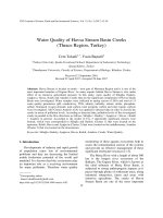
Fig. 5. Means and standard deviations of the distributions of elementary effects
of 137 factors on the total BOD load resulting from the first round of analysis.

Fig. 5 shows that there are only three important processes
that, in order of importance, have a significant contribution
to the total BOD load: brackish-pond culture (factors 68, 86,
87,124, 13 and 14), urban domestic wastewater (factors 120,
113 and 55) and industrial wastewater (factor 5).
The results obtained from the second round of the Morris
analysis (Fig. 6) show some interesting points. In contrast
with the results of the Morris analyses applied to natural system
models (Campolongo and Saltelli, 1997; Comenges and Campolongo, 2000), the rankings provided by m and s respectively

are not identical (Table 1). This can be attributed to the highly
complex combination of both linear and non-linear relationships
between the output and the input variables. However the two
rankings, which are measured by m and by the Euclidean distance from the origin in the (m, s) plane, i.e. the mean square
value, agree well (Table 1). This indicates that the mean m is
5
4.5
113

119

4

Standard deviation σ

1580

3.5
60
3

64

3

114

2.5

120

121 68

2

5

1.5

55
87
86

1

6
2 56

0.5
0
-15

124

11
79
84
66
67
62
16

65
127
126
129
131
137
136
125
128
130
135
134
133
132
115
117
116
103
102
101
105
108
107
112
118
100
104
106
111
110

109
72
71
75
81
84
89
92
91
98
97
96
95
74
73
80
79
78
77
76
83
82
88
90
94
93
99
58
57
59

63
61
23
22
21
20
19
18
17
25
27
29
31
37
36
35
43
42
47
46
45
50
54
53
52
10
12
24
26
28

30
34
33
32
41
40
39
38
44
49
48
51
1

-10

-5

0

5

10

15

Mean μ
Fig. 6. Means and standard deviations of the distributions of elementary effects
of 137 factors on the total BOD load resulting from the second round of
analysis.

T.G. Nguyen, J.L. de Kok / Environmental Modelling & Software 22 (2007) 1572e1587

113

10.81

4.19

11.59

55

8.05

1.42

8.18

124

4.85

0.64

4.89

120

3.26

2.39

4.04

68

2.56

2.01

3.25

119

2.47

4.10

4.78

87

2.40

1.07

2.63

64

2.26

3.04

3.78

114

2.14

2.57

3.34

60

2.08

3.23

3.84

3
86

1.97
1.82

3.00
0.93

3.59
2.05

121

1.03

1.99

2.24

5

0.82

1.62

1.81

56

0.63

0.42

0.76

6

0.38

0.44

0.58

122

0.30

0.19

0.35

123

0.19

0.17

0.25

13
2
133

0.17 0.13
0.22

0.15 0.40
0.43
591.3 87.33 597.7

135

233.4

132
134

66.43 242.7

60.13 19.68
46.66 16.81

63.27
49.60

Total purification capacity of domestic
wastewater treatment plants (mil. m3/day)
Percentage of urban connected
households (%)
BOD generated by 1 kg of shrimp
(kg BOD/kg shrimp)
BOD concentration of domestic
wastewater before purification (mg/l)
Spatial growth rate of shrimp pond area
(1/mil. IDR)
Production of wastewater per industrial

production value (mil. m3/mil. IDR)
Yield of the extensive shrimp culture
(ton/ha)
Time for investment of industry to take
effect (month)
Total purification capacity of industrial
water treatment plants (mil. m3/day)
Slope coefficient of the linear
relationship between investment and
production of industry (e)
Urban income (mil. IDR/cp per year)
Yield of the intensive shrimp culture
(ton/ha)
BOD concentration of industrial
wastewater before purification (mg/l)
Yearly investment on the industry
(mil. IDR/year)
Water demand for unconnected
households (m3/cp per day)
Yearly investment on shrimp
intensification (mil. IDR/year)
BOD concentration of domestic
wastewater after purification (mg/l)
BOD concentration of industrial
wastewater after purification (mg/l)
Relative growth rate of shrimp price (e)
Immigration scenario selection
Damage surface area of coral reef per
fish blast (ha/blast)
Number of fish blasts per ha per year

(blast/ha per year)
Natural growth rate of coral reef
(ha/ha per year)
Recovery rate of damage coral
(ha/ha per year)

The influential factors are listed in descending order of importance, resulting
from the second round of analysis.

a good indicator to measure the overall influence of a factor on
a certain output as argued by Morris (1991). Contrary to the results of the first round (Fig. 5), the results of the second round
(Fig. 6) do not show distinct clusters of factors. This is because
there are no dominant processes that have a much larger effect
than the others, except for the domestic wastewater discharge
(factors 113 and 55 on Fig. 6 and Table 1). To compare the effects of the industry and shrimp-culture related wastewaters,
the sum of the mean m from all factors belonging to each process
is computed. Shrimp culture contributes a value of 12.2 to the
variability of the total BOD, while industrial wastewater

contributes a value of 11.0. This small difference does not allow
a clear conclusion with regard to the order of importance of the
two processes.
Fig. 7 shows the four important factors that have an effect
on the total area of living coral from the first and second
rounds of the Morris analysis. Factors 133 (damaged surface
area of coral reef per fish blast) and 135 (the number of fish
blasts per year per ha) demonstrate that the most important
process influencing the living coral area is blast fishing. Factor
132 (natural growth rate of coral reef) and factor 134 (recovery
rate of damaged coral) play a relatively small role compared to

blast fishing. The other factors, such as the effect of suspended
sediment, are so small that they are outstripped by the effect of
a stochastic module to generate the spatial distribution of fish
blasts over the coastal sea area.
5.2. Elicitation of expert opinions
Tables 2 and 3 show the results of expert opinion aggregation of the two groups. The number of respondents answering
a specific set of questions varied depending on the objective
variable. Among the first group there were 18 and 15 respondents answering the issue of coral reef degradation and marine
pollution, respectively. The corresponding numbers among the
second groups were 7 and 8, respectively.
In Tables 2 and 3, a low average (Ave.) value indicates a high
rank of a factor, and a low standard deviation (Std.) value indicates a high degree of consensus among the respondents concerning the rank of a factor. Table 3 shows that there is
consensus among the scientific experts on the importance of
the effect of blast fishing on the living coral area. The results obtained with the stakeholder group also point to blast fishing as
the most important process, but with more variability
(Std. ¼ 1.41). Both groups identified fishing using cyanide as
the second most important factor. The two groups ranked the
400
135

350
133

300

Standard deviation σ

Table 1
Results of Morris analysis on the relative important effects of 137 factors on
the total BOD load and the living coral area

pffiffiffiffiffiffiffiffiffiffiffiffiffiffiffiffi
Factor jmj
s
m2 þ s2 Short description

1581

250
200
150
100

133
135

50
0
-700

132
134
132
38
35
39
30
25
23
24
16

15
22
40
34
33
43
42
10
36
29
7
9
64
1
6
49
20
134
37
44
13
8
5
21
27
26
2
4
41
46

61
14
47
51
17
11
48
19
28

-600

-500

-400

-300

-200

-100

0

100

200

Mean μ
Fig. 7. Means and standard deviations of the distributions of elementary effects

of 137 factors on the living coral area at the first (dot) and the second (star)
rounds of analysis.


T.G. Nguyen, J.L. de Kok / Environmental Modelling & Software 22 (2007) 1572e1587

1582

Table 2
Results of the analysis of the important factors/processes affecting the organic
pollution, elicited from local stakeholders and scientific experts (SEs)
Factor

Stakeholders

SEs (simple average) SEs (weighted average)

Ave. Std. Rank Ave.
Domestic 1.50 0.94 1
Industry 1.73 1.22 2
Shrimp
2.00 1.03 3

1.50
1.50
2.38

Std.

Rank

W. ave.

Rank

0.55
0.89
0.71

1
2
3

1.45
1.60
2.50

1
2
3

remaining four factors slightly differently. However, there is
a general agreement between the two groups about the relatively
low effect of coral reef mining for construction on living coral
area.
With respect to the sources of organic pollution of coastal
waters, the average values of domestic and industrial wastewaters (Table 2) indicate an equal importance order of the two
sources. However, for domestic wastewater, a higher consensus was obtained. When using the weighted average method
to combine expert opinions, the results show a difference between the two sources. The ranking, in descending order, is:
(1) domestic wastewater, (2) industrial wastewater, and (3)

shrimp culture wastewater. This ranking is the same as the
ranking indicated by the stakeholders.
The results in Tables 2 and 3 show that the standard deviations in the answers given by the scientific experts are generally smaller than those given by the stakeholders. This
indicates a higher degree of consensus among the SEs than
among the stakeholders. Furthermore, the difference in the average values of the two successive factors/processes is generally larger for the scientific experts than for the stakeholders
(Tables 2 and 3). The exceptions are domestic wastewater
and industrial wastewater in Table 2. This could indicate
that the SEs have more confidence to differentiate the order
of importance of the factors/processes than the stakeholders.
Assigning weights to individual expert’ answers results in
the rank of a factor which is similar to the corresponding
rank obtained by the simple average method (Tables 2 and
3). This is an indication that the simple average method is appropriate for this study.

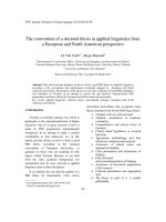
The first scenario is an extrapolation of the existing situation
(no measure), where the ban on blast fishing is not in effect
due to a number of social-economic and politic reasons. The
second scenario consists of an enforced ban on blast fishing
(with measure). An example of this situation can be found in
a study on blast fishing in Komodo National Park (Pet-Soede
et al., 1999) where about 90% of fish blasts were reduced after
a patrolling programme had been implemented. The uncertainty bounds are subject to a 95% confidence level, with a sample size of 1000 simulation runs. The similar approach is
applied for the total BOD discharge into the coastal waters.
Fig. 9 depicts the extended current scenario and the scenario
where urban wastewater treatment plants are installed, both under the assumption of 90% of connected urban households.
5.4. Parameter-Verification test
The most important factors influencing the total BOD load
and the living coral area could be identified in the first round
of the Morris analysis (Figs. 5 and 7). The order of importance
of these factors is affected by the model as well as the analyst’s

errors, as explained previously. To reduce the analyst’s error in
estimating the ranges of parameters and inputs, a comparison of
the results of the first round and the opinions of the local stakeholders and experts were used as a the starting point for the investigation. For the total BOD load, all parameters and inputs
which belong to the three important processes, as suggested
by the local stakeholders and experts, were subject to a careful
examination. A number of refinements on the uncertainty range
of these parameters and inputs have been made. For example,
the literature study (Fung-Smith and Briggs, 1996; Otte,
1997) revealed an overestimation of factor 124 (amount of
BOD generated per kg of shrimps). In contrast, industrial investment (factor 5) was overlooked by assigning it a too small
range. Similarly for the living coral area, factor 133 (damaged
16000
14000
12000

The uncertainty propagations of the input factors to the living coral area have been compared for two scenarios (Fig. 8).
Table 3
Results of the analysis of the important factors/processes affecting the living
coral area, elicited from local stakeholders and scientific experts (SEs)
Factor

Suspended sediment
Blast
Cyanide
Natural growth
Recover
Mining

Stakeholders

SEs (simple
average)

SEs (weighted
average)

Ave. Std. Rank Ave. Std. Rank W. ave.

Rank

2.74
2.00
2.17
2.22
2.61
2.95

3
1
2
4
6
5

0.73
1.41
1.47
1.26
1.42
1.35

5
1
2
3
4
6

2.29
1.29
2.00
2.57
3.00
2.71

0.95
0.49
1.15
0.98
1.15
0.95

3
1
2
4
6
5

2.29

1.35
1.97
2.73
3.13
2.85

Living coral area (ha)

5.3. Uncertainty analysis

10000
8000
6000
4000
2000
0
1995

2000

2005

2010

2015

2020

Time (year)
Fig. 8. Results of the Monte Carlo uncertainty analyses on the living coral area

for the two scenarios: (a) full enforcement of a ban on blast fishing (dotted
lines, 95% confidence bounds; and ,, mean) and (b) without this measure
(solid lines, 95% confidence bounds; B, mean).


T.G. Nguyen, J.L. de Kok / Environmental Modelling & Software 22 (2007) 1572e1587
300

Total BOD load (ton/day)

250

200

150

100

50

0
1995

2000

2005

2010

2015

2020

Time (year)
Fig. 9. Results of the Monte Carlo uncertainty analyses on the total BOD load to
the coast for the two scenarios: (a) with the implementation of wastewater treatment plants of 145,000 m3/day (dotted lines, 95% confidence bounds; ,, mean),
and (b) without this measure (solid lines, 95% confidence bounds; B, mean).

surface area of coral reef per fish blast) was overestimated
whereas the factor 135 (number of fish blasts per ha per year)
was underestimated (Pet-Soede et al., 1999). The natural
growth rate of coral (factor 132) and the recovery rate of damaged coral (factor 134) were also adjusted according to Saila
et al. (1993) and Fox et al. (2003). After refining all the ranges
of the important factors discovered in the first round of the Morris analysis and the local stakeholders and experts’ opinions,
the second round was carried out. The results are shown in
Fig. 6, for BOD load and Fig. 7 (star) for the total area of living
coral. Fig. 6 shows that the percentage of urban households
connected to the water supply network (factor 55) is a strong
determinant of the total BOD load. This percentage was treated
as a constant parameter in RaMCo. It might need to be converted to a variable which is driven by socio-economic factors
and policy options in RaMCo.
5.5. Behaviour-Anomaly test
As shown in Figs. 5 and 6 the order of importance of the relevant processes has changed, in comparison to the first round of
the Morris analysis. There is an agreement between the model
and the stakeholders/experts (Table 2) with respect to the most
important source of organic pollution, domestic wastewater discharge (factors 113, 55, 120). However, there is a disagreement
about the order of importance of industrial wastewater (factors
119, 64, 114) and shrimp culture wastewater (factors 124, 68,
87). There are three possible explanations for this difference.
First, the shrimp-pond area is located along the coastal line

whereas the domestic and industrial wastewater discharges
originate from the city of Makassar. This may distort the perception of the experts with regard to the order of magnitude
of the pollutant sources. Second, the assumption on the linear
relationship between shrimp production and the production of
the BOD load may not be valid. The equation employed in

1583

RaMCo is: Q(t) ¼ CA(t)I(t), where Q(t) is total BOD load
(ton/year), C is the amount of BOD generated by a kilogram
of shrimp (kg/kg), A(t) is the area of shrimp culture at year t
(ha), and I(t) is the yield of shrimp at year t (ton/ha). Empirical
data and research on this relationship are lacking in the scientific literature, so it requires further investigation. Third, the variability of the BOD concentration of the industrial wastewater is
very large and strongly dependent on the types of industry prevailing in the study area. The analysis of BOD concentration of
industrial wastewater was based on a previous investigation of
industrial sectors carried out by JICA (1994). According to the
authors, the research outcomes should be interpreted carefully
since they were derived from a very limited measurement.
Therefore, more research on this topic should be conducted.
Obvious flaws in the model cannot be found in this case, but
outcomes of the test justify further research.
For the important factors influencing the area of living coral,
there is an agreement that blast fishing (factors 133, 135) is the
most influential process. A comparable result is obtained on the
natural growth rate (factor 132) and the recovery rate of damaged coral (factor 134) (Fig. 7 and Table 3). However, a shortcoming of RaMCo is that it does not include the process of
fishing using poisonous substances, which is regarded as being
more important than the natural growth rate and the recovery
rate by both stakeholders and experts. The effect of suspended
sediment on the living coral is ranked differently by stakeholders and experts (Table 3). The results of the model agree
more with the stakeholders’ assessments. Nevertheless, the differences call for an in-depth investigation of the effect of the

suspended sediment on the living coral for the study area.
5.6. Policy-Sensitivity test
As depicted by Fig. 8, the difference between the extended
current situation and the situation with an enforcement of the
ban on blast fishing is clear. There is no overlap between the
confidence bounds. The time series of the predicted mean
values are significantly different in terms of trend lines. This
gives the decision makers more confidence in using the model.
For the BOD load (Fig. 9), there is a large overlap between
the two scenarios where urban wastewater treatment plants are
installed or not. The difference between the two time series of
the predicted mean values of the total BOD load is small compared with the overlap of the confidence bounds after the year
2005. In addition, the trend lines of the predicted mean values
in two situations are almost the same. This suggests that this
measure should not be implemented separately but combined
with other measures, such as the installation of industrial
wastewater treatment plants and water treatment structures
for shrimp pond area. In this case, this test does not increase
the confidence of the decision makers.
6. Discussion
In this paper, the concepts of validity and validation of ISMs
have been defined. A conceptual framework for ISM validation
and the detailed steps have been presented. This framework and


1584

T.G. Nguyen, J.L. de Kok / Environmental Modelling & Software 22 (2007) 1572e1587

the procedure reflect the philosophical position taken in this paper, which lies somewhere between objectivism (in the

sense that there is an ultimate truth) and relativism (one model
is as good as another), beyond rationalism and positive empiricism. Based on this position, we consider an ISM as a tool which
is designed for specified purposes. The model validation is considered to be a process, which should take these purposes into
account.
The examples clearly demonstrate that the Morris (1991)
method can be a valuable tool for the validation of an integrated systems model. First, it helps to pinpoint the parameters, inputs and measures that need careful investigations in
the process of model validation. Second, it allows the endusers of a model to judge qualitatively the validity of the hypotheses embedded in the model. Third, it helps to find the
backbone of a model, on which the validation should be based.
The current method of the expert elicitation does not take
into account two aspects of the expert opinion, namely, bias
and inconsistency. Nevertheless, it is simple, informative,
time and cost effective. Given its purpose as an exploratory
tool, it is acceptable for this type of applications. Alternative
methods such as analytical hierarchy process and adaptive
conjoint analysis may further improve the credibility of the
results.
The approach to the validation of integrated systems models
presented in this paper is a combination of the sensitivity and
uncertainty analyses with the three validation tests of system
dynamics models proposed by Forrester and Senge (1980). Taking into account the increasing difficulties in collecting data for
empirical validation of ISMs, the current approach is one of the
possible ways to get out of ‘‘the impasse’’ mentioned by Beck
and Chen (2000). Our argument for the current approach is that
one main purpose of ISM validation is to show transparently
both the strengths and weaknesses of a model to its intended
users. To the model developers, validation can reveal flaws in
the model, from which they may see a need to improve or rebuild the model. To the analysts, validation can provide the necessary information to facilitate the process of calibration for
other applications, and analysis of the results before transferring them to the decision makers. Finally, validation gives decision makers confidence in using the model results to support

their decision-making processes. This argument is in line with

the current view that the validation of ISMs is a process, not a final product of integrated assessment (Parker et al., 2002); and
one important component of it is the adaptive feedback between
stakeholders and researchers (Jakeman and Letcher, 2003).
The three tests presented in this paper can be used as the
first steps in the process of establishing the validity of an
ISM. They have diagnostic power. A new approach, in which
a hypothesised system is built and compared with the model
system, is presented in Nguyen et al (2007). Within this
approach, the validity of the two systems is evaluated in terms
of the capability to fulfil a specified task. This testing approach
has constructive power, and helps to overcome the problems of
system openness, uncertain future context and scarcity of field
data. Another testing procedure for model validation when observed data are available to a limited extent is presented in
Nguyen (2005). This testing procedure contains three tests
(pattern replication test, behaviour accuracy test and extreme
policy test), which were applied to validate the fisheries model
incorporated in RaMCo.
In accordance with Rykiel (1996) and others (e.g. Oreskes,
1998; Sterman, 2002; Refsgaard and Henriksen, 2004), we
conclude that the validity of any model, in the sense of scientific hypothesis testing, is not feasible. The validity of a model
is always provisional and based on the availability of field data
and knowledge of the real system against which the model can
be tested. However, model validation is a legitimate activity
required to improve our understanding and to guide our management decisions.

Acknowledgements
The authors wish to thank Ms Tessa Hoffman for her careful work on preparing, distributing, and collecting the questionnaires. The authors are grateful to prof. dr. A. Noor and
prof. dr. D. Ahmad for arranging the workshops and inviting
the respondents. The research was partially supported by
The Netherlands Foundation for The Advancement of Tropical

Research (WOTRO). Anonymous reviewers of the paper are
gratefully acknowledged.

Appendix A. Example of the questionnaire
In order to make the RaMCo a useful tool in practice, we would like to have your valuable contributions to the process of model validation by thoroughly filling
this questionnaire.
No.

Question

A
B

What is your name?
What is your title?
(e.g. Prof., Dr., Deputy head of the department)
Where do you work?
(e.g. Department of Forestry, UNHAS University)
Land use
Marine water
Marine
management
quality
fisheries

C
D: What is/are your
field(s) of expertise?
E: How long have you been
working on these field(s)?

Marine
ecology

Answer

Other
(please specify)


T.G. Nguyen, J.L. de Kok / Environmental Modelling & Software 22 (2007) 1572e1587

1585

A.1 Coral reefs
In this section, you are asked for the relative importance order of factors and processes that have effects on coral reefs. Please answer these questions by
marking them in appropriate places.
No.

Question

Answer

33

YES
NO
Information gathered
in practice

35

Do you have knowledge
of the coral reef?
Where do you obtain your knowledge
to answer these questions?
(Multiple answers possible)
Are you interested in coral reef?

No.

Factor/process

36

The impact of suspended sediment
on coral reefs
The fisheries using dynamite
Cyanide fishing
The expansion of coral reef area
Recovery rate of damaged coral
The use of coral for the supply
construction

34

37
38
39
40

41

Please go on with question 34
Please go on with question 47
Information gathered through research

Very interested
Interested
Moderate
Little
Not at all
1: extremely
important

2: very
important

3: important

4: not so
important

5: not
important at all

6: I have no idea

There also can be some factors/processes we overlooked. Please add them to the list and explain how important these factor/processes are, by giving them a ranking
too.
No.

42
43

Factor/process

1

2

3

4

5

6

44
45
46

Appendix B. Weighting factors for aggregation of expert opinions
Table B.1
Weighting factor for professional title (PT)
Stakeholders/policy makers

Research experts

Weighting factor

Heads of an institution
Head of a department
Staff member

Professor
Doctor
Master of Science/Engineer

2.0
1.5
1.0

Table B.2
Weighting factor for source of knowledge (SK)
Source of knowledge

Weighting factor

Information gathered
from practice
Information gathered
from research
Information gathered
from both practice and research

1.0
1.0
2.0

1586

T.G. Nguyen, J.L. de Kok / Environmental Modelling & Software 22 (2007) 1572e1587

Table B.3
Weighting for years of experience (YE)
Time active in field of expertise

Weighting factor

0e5 years
5e10 years
10e15 years
15e20 years
More than 20 years

0
0.5
1.0
1.5
2.0

Table B.4
Weighting factor for level of interest (LI)
Level of interest

Weighting factor

Very interested
Interested

Moderate
Little interested
Not at all interested

2
1.5
1.0
0.5
0.0

References
Ayyub, B.M., 2001. A Practical Guide on Conducting Expert-Opinion Elicitation of Probabilities and Consequences for Corp Facilities. IWR Report
01-R-1. Prepared for US Army Corps of Engineering. Institute for Water
Resources, Alexandria, VA. 22315e3868.
Barlas, Y., 1994. Model validation in system dynamics. Proceedings of the
1994 International System Dynamics Conference. Methodological Issues.
Stirling, Scotland, pp. 1e10.
Beck, M.B., Chen, J., 2000. Assuring the quality of model designed for predictive purposes. In: Saltelli, A., Chan, K., Scott, E.M. (Eds.), Sensitivity
Analysis. Wiley, Chichester, pp. 401e420.
Bhatnagar, R.N., Kanal, L., 1992. Models of enquiry and formalisms for approximate reasoning. In: Zadeh, L.A., Kacprzyk, J. (Eds.), Fuzzy Logic
for the Management of Uncertainty. John Wiley & Sons, pp. 29e54.
Campolongo, F., Saltelli, A., 1997. Sensitivity analysis of an environmental
model: an application of different analysis methods. Reliability Engineering & System Safety 57, 49e69.
Cocks, A.T., Rodgers, I.R., Skeffington, R.A., Webb, A.H., 1998. The limitations of integrated assessment modelling in developing air pollution control policies. Environmental Pollution 102, 635e639.
Comenges, J.-M.Z., Campolongo, F., 2000. An application of sensitivity analysis to fish population dynamics. In: Saltelli, A., Chan, K., Scott, E.M.
(Eds.), Sensitivity Analysis. Wiley, Chichester, pp. 367e383.
Cooke, R.M., 1991. Experts in Uncertainty: Opinion and Subjective Probability in Science. Oxford University Press, New York.
Cornelissen, A.M.G., Berg, J.V.D., Koops, W.J., Kaymak, U., 2003. Elicitation
of expert knowledge for fuzzy evaluation of agricultural production systems. Agriculture, Ecosystems and Environment 95, 1e18.
De Kok, J.L., Wind, H.G., 2002. Rapid assessment of water systems based on

internal consistency. Journal of Water Resources Planning and Management 128 (4), 240e247.
Dery, R., Landry, M., Banville, C., 1993. Revisiting the issue of model validation in OR: an epistemological view. European Journal of Operational Research 66, 168e183.
Dowlatabadi, H., 1995. Integrated assessment models of climate change: an incomplete overview. Energy Policy 23 (4/5), 289e296.
Forrester, J.W., Senge, P.M., 1980. Tests for building confidence in system dynamics models. In: Legasto Jr. A.A., Forrester, J.W., Lyneis, J.M. (Eds.),
System Dynamics. TIMS Studies in Management Sciences, Vol. 14. North
Holland, pp. 209e228.
Fox, H.E., Pet, J.S., Dahuri, R., Caldwell, R.L., 2003. Recovery in rubble
fields: long-term impacts of blast fishing. Marine Pollution Bulletin 46,
1024e1031.
Fung-Smith, S.J., Briggs, M.R.P., 1996. Water quality and nutrient discharge
of intensive marine shrimp ponds in Thailand and their relationships to

pond productivity. Institute of Aquaculture. University of Stirling, Stirling,
FK9 4 LA, Scotland, UK.
Hoekstra, A.Y., 1998. Perspectives on Water: A Model-based Exploration of
the Future. International Books, Utrecht, The Netherlands.
Hulme, M., Raper, C.B.S., 1995. An integrated framework to address climate
change (ESCAPE) and further developments of the global and regional climate modules (MAGICC). Energy Policy 23 (4/5), 347e355.
Iman, R.L., Helton, J.C., 1988. An investigation of uncertainty and sensitivity
analysis techniques for computer models. Risk Analysis 8 (1), 71e90.
Jakeman, A.J., Letcher, R.A., 2003. Integrated assessment and modelling: features, principles and examples for catchment management. Environmental
Modelling & Software 18, 491e501.
Janssen, M., de Vries, B., 1998. The battle of perspectives: a multi-agent
model with adaptive responses to climate change. Ecological Economics
26, 43e65.
Janssen, M., De Vries, B., 1999. Global modeling: managing uncertainty, complexity and incomplete information. In: van Dijkum, C., de Tombe, D., van
Kuijck, E. (Eds.), Validation of Simulation Models. SISWO, Amsterdam,
pp. 45e69.
JICA, 1994. Master Plan and Feasibility Study on Wastewater and Solid Waste
Management for The City of Ujung Pandang in The Republic of Indonesia.

Progress Report No. 1. Pacific Consultants International, Tokyo and Yachiyo Engineering Co. LTD, Tokyo.
Kirchner, J.W., Hooper, R.P., Kendall, C. et al., 1996. Testing and validating environmental model. The Science of the Total Environment 183,
33e47.
Kleijnen, J.P.C., 1995. Verification and validation of simulation models. European J. Operational Research 82, 145e162.
Kleindorfer, J.B., O’Neill, L., Ganeshan, R., 1998. Validation in simulation:
various positions in the philosophy of science. Management Science 44
(8), 1087e1099.
Konikow, L.F., Bredehoeft, J.D., 1992. Ground-water models cannot be
validated. Advances in Water Resources 15 (1), 75e83.
Kuhn, T.S., 1970. The Structure of Scientific Revolutions, second ed. University of Chicago Press, Chicago, IL.
Mitchell, P.L., 1997. Misuse of regression for empirical validation of models.
Agricultural Systems 54 (3), 313e326.
Morgan, M.G., Henrion, M., 1990. Uncertainty: A Guide to Dealing with
Uncertainty in Quantitative Risk and Policy Analysis. Cambridge University
Press.
Morris, D.M., 1991. Factorial sampling plans for preliminary computational
experiment. Technometrics 33 (2), 161e174.
Nguyen, T.G., 2005. A methodology for validation of integrated systems
models with an application to coastal-zone management in south-west Sulawesi. PhD dissertation. University of Twente, The Netherlands. ISBN:
90-365-2227-7.


T.G. Nguyen, J.L. de Kok / Environmental Modelling & Software 22 (2007) 1572e1587
Nguyen, T.G., De Kok, J.L., Titus, M., 2007. A new approach to testing an
integrated water systems model using qualitative scenarios. Environmental
Modelling & Software 22 (11), 1557e1571.
Oreskes, N., 1998. Evaluation (not validation) of quantitative models. Environmental Health Perspectives 106 (6), 1453e1460.
Oreskes, N., Frechette, K.S., Belitz, K., 1994. Verification, validation, and confirmation of numerical models in the earth sciences. Science 263, 641e646.
Otte, Y., 1997. Impact of shrimp culture development on the water quality at
the Southwest coast of Sulawesi. In: Reports Environmental Studies no.

148. Department of Environmental Studies, Faculty of Sciences, University of Nijmegen, The Netherlands.
Parker, P., Letcher, R., Jakeman, A.J., Beck, M.B., Harris, G., Argent, R.M.,
Hare, M., Pahl-Wostl, C., Voinov, A., Janssen, M., et al., 2002. Progress
in integrated assessment and modeling. Environmental modelling & Software 17, 209e217.
Pet-Soede, C., Cesar, H.S.J., Pet, J.S., 1999. An economic analysis of blast fishing on Indonesian coral reefs. Environmental Conservation 26 (2), 83e93.
Popper, K.R., 1959. The Logic of Scientific Discovery. Hutching and Son
Company, London, UK.
Reckhow, K.H., Chapra, S.C., 1983. Confirmation of water quality models.
Ecological Modelling 20, 113e133.
Refsgaard, J.C., Henriksen, H.J., 2004. Modelling guidelines-terminology and
guiding principles. Advances in Water Resources 27, 71e82.
Rykiel, E.J., 1996. Testing ecological models: the meaning of validation. Ecological Modelling 90, 229e244.
Saila, S.B., Kocic, V.Lj., McManus, J.W., 1993. Modelling the effects of destructive fishing practices on tropical coral reefs. Marine Ecology Progress
Series 94, 51e60.
Sensitivity Analysis. In: Saltelli, A., Chan, K., Scott, M. (Eds.), Probability
and Statistics Series. John Wiley & Sons, p. 475.

1587

Saltelli, A., Scott, M., 1997. Guest editorial: The role of sensitivity
analysis in the corroboration of models and its link to model structural
and parametric uncertainty. Realiability Engineering and System Safety
57, 1e4.
Sargent, R.G., 1991. Simulation model verification and validation. Proceedings of the 1991 Winter Simulation Conference, pp. 37e47.
Scholten, H., Cate, A.J.U., 1999. Quality assessment of the simulation modeling process. Computers and Electronics in Agricultures 22, 199e208.
Shannon, E.R., 1981. Tests for verification and validation of computer simulation models. Proceedings of the 1998 Winter Simulation Conference,
pp. 573e577.
Tarantola, S., Jesinghaus, J., Poulamaa, M., 2000. Global sensitivity analysis: a quality assurance tool in environmental policy modelling. In: Saltelli, A., Chan, K., Scott, E.M. (Eds.), Sensitivity Analysis. Wiley,
Chichester, pp. 385e397.
Turner, R.K., 2000. Integrated natural and socio-economic science in coastal

management. Journal of Marine Systems 25, 447e460.
Van der Fels-Klerx, H.J., Horst, H.S., Dijkhuizen, A.A., 2000. Risk factors for
bovine respiratory disease in dairy youngstock in The Netherlands: the perception of experts. Livestock Production Science 66, 35e46.
Uljee, I., Engelen, G., White, R., 1996. RAMCO Demo Guide. Modelling and
Simulation Research Group, Research Institute for Knowledge Systems
BV, PO Box 463, 6200 AL Maastricht, The Netherlands.
Zio, E., 1996. On the use of the analytical hierarchy process in the aggregation of expert judgments. Reliability Engineering and System Safety 53,
127e138.
Zio, E., Apostolakis, G.E., 1997. Accounting for expert-to-expert variability:
a potential source of bias in performance assessments of high-level
radioactive waste repositories. Annals of Nuclear Energy 24 (10),
751e762.