On integral operators generatedby the fourier transform and a reflection

Memoirs on Differential Equations and Mathematical Physics
Volume 66, 2015, 7–31

L. P. Castro, R. C. Guerra, and N. M. Tuan

ON INTEGRAL OPERATORS GENERATED
BY THE FOURIER TRANSFORM AND A REFLECTION

Dedicated to the memory of Professor Boris Khvedelidze (1915–1993)
on the 100th anniversary of his birthday


Abstract. We present a detailed study of structural properties for certain algebraic operators generated by the Fourier transform and a reection. First, we focus on the determination of the characteristic polynomials
of such algebraic operators, which, e.g., exhibit structural dierences when
compared with those of the Fourier transform. Then, this leads us to the
conditions that allow one to identify the spectrum, eigenfunctions, and the
invertibility of this class of operators. A Parseval type identity is also obtained, as well as the solvability of integral equations generated by those
operators. Moreover, new convolutions are generated and introduced for
the operators under consideration.
2010 Mathematics Subject Classication. 42B10, 43A3, 44A20,
47A05.
Key words and phrases. Characteristic polynomials, Fourier transform, reection, algebraic integral operators, invertibility, spectrum, integral equation, Parseval identity, convolution.

ềặẫệè. ĩ òềèẽẫẩ ìệềẫể ềỉèẫẩ ềấậẫể
ẽéềễẽềẫẩ òềèẽỉẫậẫ ặẽẫềẩẫ ậềệậẫ ẽéềễẽềẫể
ểễềệỉễệềệậẫ ẩẫểẫể ễậệề ấậể. éẫềậ ềẫẫ, ệề èỏẫậệậẫ ểẩẫ ậềệậẫ ẽéềễẽềẫểẩẫể èỏểẫẩậẫ éẽậẫẽèẫể ểặềặ, ềẽèậẫí ỏể
ểễềệỉễệềệậ ểỏể ìệềẫể ềỉèểẩ ềẫẩ.
èể èẫềẩ éẫềẽẩ, ềẽèậẫí ểệậể èẽíèể èẽỏẫẽẩ ểéỉễềẫể, ểấệẩềẫẫ ìệíẫẫể è ấậểẫ ềệẫ
ẽéềễẽềẫể ẫễẫìẫíẫề. èẫệậẫ éềểậẫể ễẫéẫể ẫẫẽ ểòậẫậẫ è ẽéềễẽềẫẩ òềèẽỉèẫậẫ ẫễềậệềẫ ễẽậẫể èẽỏểẽ. ỏẫậệậẫ ẽéềễẽềẫểẩẫể
èẽễẫậẫ ỏậẫ ỏẫể ẽéềễẽềẫể í.

On Integral Operators Generated by the Fourier Transform and a Reflection

9

1. Introduction
In several types of mathematical applications it is useful to apply more
than once the Fourier transformation (or its inverse) to the same object, as
well as to use algebraic combinations of the Fourier transform. This is the
case e.g. in wave diffraction problems which – although being initially modeled as boundary value problems – can be translated into single equations
by applying operator theoretical methods and convenient operators upon
the use of algebraic combinations of the Fourier transform (cf. [8–10]). Additionally, in such processes it is also useful to construct relations between
convolution type operators [7], generated by the Fourier transform, and
some simpler operators like the reflection operator; cf. [5, 6, 11, 21]. Some
of the most known and studied classes of this type of operators are the
Wiener–Hopf plus Hankel and Toeplitz plus Hankel operators.
It is also well-known that several of the most important integral transforms are involutions when considered in appropriate spaces. For instance,
the Hankel transform J, the Cauchy singular integral operator S on a
closed curve, and the Hartley transforms (typically denoted by H1 and H2 ,
see [2–4, 17]) are involutions of order 2. Moreover, the Fourier transform F
and the Hilbert transform H are involutions of order 4 (i.e. H4 = I, in this
case simply because H is an anti-involution in the sense that H2 = −I).
Those involution operators possess several significant properties that are
useful for solving problems which are somehow characterized by those operators, as well as several kinds of integral equations, and ordinary and partial
differential equations with transformed argument (see [1, 15, 16, 18, 20, 22–
26]).
Let W : L2 (Rn ) → L2 (Rn ) be the reflection operator defined by
(W φ)(x) := φ(−x),
and let now ⟨ · , · ⟩L2 (Rn ) denote the usual inner product in L2 (Rn ). Moreover, let F denote the Fourier integral operator given by
∫

1
(F f )(x) :=
e−i⟨x,y⟩ f (y) dy.
n
(2π) 2
Rn

In view of the above-mentioned interest, in the present work we propose
a detailed study of some of the fundamental properties of the following
operator, generated by the operators I (identity operator), F and W :
T := aI + bF + cW : L2 (Rn ) → L2 (Rn ),

(1.1)

where a, b, c ∈ C. In very general terms, we can consider the operator T as
a Fourier integral operator with reflection which allows to consider similar
operators to the Cauchy integral operator with reflection (see [12–14, 19]
and the references therein). Anyway, it is also well-known that F 2 = W .
In this paper, the operator T , together with its properties, can be seen as a
starting point to further studies of the Fourier integral operators with more
general shifts that will be addressed in the forthcoming papers.


10

L. P. Castro, R. C. Guerra, and N. M.Tuan

The paper is organized as follows. In the next section, we will justify
that T is an algebraic operator and we will deduce their characteristic polynomials for distinct cases of the parameters a, b and c. Then, the conditions
that allow to identify the spectrum, eigenfunctions, and the invertibility of

the operator are obtained. Moreover, Parseval type identities are derived,
and the solvability of integral equations generated by those operators is
described. In addition, new operations for the operators under consideration are introduced such that they satisfy the corresponding property of the
classical convolution.

2. Characteristic Polynomials
In order to have some global view on corresponding linear operators, we
start by recalling the concept of algebraic operators.
An operator L defined on the linear space X is said to be algebraic if
there exists a non-zero polynomial P (t), with variable t and coefficients in
the complex field C, such that P (L) = 0. Moreover, the algebraic operator
L is said be of order N if P (L) = 0 for a polynomial P (t) of degree N , and
Q(L) ̸= 0 for any polynomial Q of degree less than N . In such a case, P
is said to be the characteristic polynomial of L (and its roots are called the
characteristic roots of L). As an example, for the operators J, S, H1 , H2
and H, mentioned in the previous section, we may directly identify their
characteristic polynomials in the following corresponding way:
PJ (t) = t2 − 1;
PH1 (t) = t2 − 1;

PS (t) = t2 − 1;

PH2 (t) = t2 − 1;

PH (t) = t2 + 1.

As above mentioned, it is well-known that the operator F is an involution
of order 4 (thus F 4 = I, where I is the identity operator in L2 (Rn )). In other
words, F is an algebraic operator which has a characteristic polynomial
given by PF (t) = t4 − 1. Such polynomial has obviously the following four

characteristic roots: 1, −i, −1, i.
We will consider the following four projectors correspondingly generated
with the help of F :
1
(I
4
1
P1 = (I
4
1
P2 = (I
4
1
P3 = (I
4
P0 =

+ F + F 2 + F 3 ),
+ iF − F 2 − iF 3 ),
− F + F 2 − F 3 ),
− iF − F 2 + iF 3 ),


On Integral Operators Generated by the Fourier Transform and a Reflection

and that satisfy the identities


for j, k = 0, 1, 2, 3,
Pj Pk = δjk Pk

P0 + P1 + P2 + P3 = I,


F = P0 − iP1 − P2 + iP3 ,
where
δjk

11

(2.1)

{
0, if j ̸= k,
=
1, if j = k.

Moreover, we have
F 2 = P0 − P1 + P2 − P3 ,
4

F = P0 + P1 + P2 + P3 = I.

(2.2)
(2.3)

It is also clear that
αP0 + βP1 + γP2 + δP3 = 0
if and only if
α = β = γ = δ = 0.
Having in mind this property, in the sequel, for denoting the operator

A = αP0 + βP1 + γP2 + δP3 ,
we will use the notation (α; β; γ; δ) = A.
Obviously, An = (αn ; β n ; γ n ; δ n ), for every n ∈ N, where we admit that
0
A = I.
Theorem 2.1. Let us consider the operator
T = aI + bF + cW, a, b, c ∈ C.

(2.4)

The characteristic polynomial of this T is:
(i)
PT (t) = t2 − 2at + (a2 − c2 )

(2.5)

b = 0 and c ̸= 0;

(2.6)

if and only if
(ii)

[
]
[
]
PT (t) = t3 − (3a + c) + ib t2 + 3(a2 − c2 ) + 2a(c + ib) t
[
]

+ − a3 − ia2 b − a2 c − 3b2 c + 3ac2 + ibc2 + c3
if and only if
bc ̸= 0 and

(

)
b
b
c = (1 − i) or c = − (1 + i) ;
2
2

(2.7)

(2.8)


12

L. P. Castro, R. C. Guerra, and N. M.Tuan

(iii)

[
]
[
]
PT (t) = t3 + − (3a + c) + ib t2 + 3(a2 − c2 ) + 2a(c − ib) t
[

]
+ − a3 + ia2 b − a2 c − 3b2 c + 3ac2 − ibc2 + c3
if and only if

(

bc ̸= 0 and

)
b
b
c = (1 + i) or c = − (1 − i) ;
2
2

(2.9)

(2.10)

(iv)
PT (t) = t4 − 4at3 + (6a2 − 2c2 )t2 + (−4a3 − 4b2 c + 4ac2 )t
+ (a2 − c2 )2 + b2 (4ac − b2 )
if and only if


b

c ̸= (1 − i),




2



c ̸= − b (1 + i),
2
b


c
=
̸
(1 + i),


2



c ̸= − b (1 − i)
2

(2.11)

(2.12)

and b ̸= 0.
Proof. We can write the operator T in the following form:
T = a(P0 + P1 + P2 + P3 ) + b(P0 − iP1 − P2 + iP3 )

+ c(P0 − P 1 + P2 − P3 )
= (a + c + b)P0 + (a − c − ib)P1
+ (a + c − b)P2 + (a − c + ib)P3
= (a + c + b; a − c − ib; a + c − b; a − c + ib).

(2.13)

In order to determine the characteristic polynomial of the operator T , for
each one of the cases, we may begin by considering a polynomial of order
2, that is, PT (t) = t2 + mt + n. In fact, a polynomial of order 1 is the
characteristic polynomial of the operator T if and only if b = 0 and c = 0,
but in this case, we obtain the trivial operator T = aI. That PT (t) is the
characteristic polynomial of T if and only if PT (T ) = 0 and if there does
not exist any polynomial Q with deg(Q) < 2 such that Q(T ) = 0.
Moreover, the condition PT (T ) = 0 is equivalent to

(a + c + b)2 + m(a + c + b) + n = 0,



(a − c − ib)2 + m(a − c − ib) + n = 0,

(a + c − b)2 + m(a + c − b) + n = 0,



(a − c + ib)2 + m(a − c + ib) + n = 0.


On Integral Operators Generated by the Fourier Transform and a Reflection

13

The solution of this system is b = 0 and c = 0 (but in this case, we obtain
the trivial operator T = aI) or that

b = 0,



c ̸= 0,

m = −2a,



n = a2 − c2 .
So, if b = 0 and c ̸= 0, then PT (t) = t2 − 2at + a2 − c2 . Indeed, by using
the operator T written in the above form (2.13), it is possible to verify that
PT (T ) = 0:
T 2 − 2aT + (a2 − c2 )I
(
)
= (a + c)2 ; (a − c)2 ; (a + c)2 ; (a − c)2 − 2a(a + c; a − c; a + c; a − c)
+ (a2 − c2 )(1; 1; 1; 1) = (0; 0; 0; 0).
Now, we will prove that there does not exist any polynomial Q with
deg(Q) < 2 such that Q(T ) = 0.
Suppose that there exists a polynomial Q, defined by Q(t) = t + m, that
satisfies Q(T ) = 0. In this case, we would have the following system of
equations:

{
(a + c) + m = 0,
(a − c) + m = 0,
which is equivalent to c = 0, but this is not the case under the conditions
imposed before.
Conversely, assume that PT (t) = t2 − 2at + (a2 − c2 ) is the characteristic
polynomial of T . Thus, PT (T ) = 0, which is equivalent to
0 = T 2 − 2aT + (a2 − c2 )I
(
)
= (a + c)2 ; (a − c)2 ; (a + c)2 ; (a − c)2
− 2a(a + c; a − c; a + c; a − c) + (a2 − c2 )(1; 1; 1; 1).
This implies that b = 0 and c = 0 (which is the case of the trivial
operator) or that b = 0. So, case (i) is proved.
To obtain the characteristic polynomial for the other cases, we have to
consider polynomials with degree greater than 2. So, let us consider a
polynomial PT (t) = t3 + mt2 + nt + p and repeat the same procedure. Thus,
PT (T ) = 0 is equivalent to

(a + c + b)3 + m(a + c + b)2 + n(a + c + b) + p = 0,



(a − c − ib)3 + m(a − c − ib)2 + n(a − c − ib) + p = 0,

(a + c − b)3 + m(a + c − b)2 + n(a + c − b) + p = 0,



(a − c + ib)3 + m(a − c + ib)2 + n(a − c + ib) + p = 0.

14

L. P. Castro, R. C. Guerra, and N. M.Tuan

This system has as solutions b = 0 and c = 0 (in this case, we obtain the
operator T = aI) or b = 0 and c ̸= 0 (but for this case, the characteristic
polynomial is of order 2 – case (i)) or


b ̸= 0,




b
b


c = 2 (1 − i) or c = − 2 (1 + i),
[
]
m = − (3a + c) + ib ,




n = 3(a2 − c2 ) + 2a(c + ib),




p = −a3 − ia2 b − a2 c − 3b2 c + 3ac2 + ibc2 + c3
or



b ̸= 0,




b
b


c = 2 (1 + i) or c = − 2 (1 − i),
[
]
m = − (3a + c) + ib ,




n = 3(a2 − c2 ) + 2a(c − ib),



p = −a3 + ia2 b − a2 c − 3b2 c + 3ac2 − ibc2 + c3 .
So,

• if c =

b
2

(1 − i) or c = − 2b (1 + i), then
[
]
[
]
PT (t) = t3 − (3a + c) + ib t2 + 3(a2 − c2 ) + 2a(c + ib) t
[
]
+ − a3 − ia2 b − a2 c − 3b2 c + 3ac2 + ibc2 + c3 ;

• If c =

b
2

(1 + i) or c = − 2b (1 − i), then
[
]
[
]
PT (t) = t3 − (3a + c) + ib t2 + 3(a2 − c2 ) + 2a(c − ib) t
[
]
+ − a3 + ia2 b − a2 c − 3b2 c + 3ac2 − ibc2 + c3 .

If we consider the case c = 2b (1 − i), by using the operator T written in
the above form (2.13), we can prove that PT (T ) = 0. Indeed,
[
]
[
]
T 3 − (3a + c) + ib T 2 + 3(a2 − c2 ) + 2a(c + ib) T
[
]
+ − a3 − ia2 b − a2 c − 3b2 c + 3ac2 + ibc2 + c3 I
(
)
= [a + c + b]3 ; [a − c − ib]3 ; [a + c − b]3 ; [a − c + ib]3
[
](
)
− (3a + c) + ib [a + c + b]2 ; [a − c − ib]2 ; [a + c − b]2 ; [a − c + ib]2
[
]
+ 3(a2 − c2 ) + 2a(c + ib) (a + c + b; a − c − ib; a + c − b; a − c + ib)
[
]
+ − a3 − ia2 b − a2 c − 3b2 c + 3ac2 + ibc2 + c3 (1; 1; 1; 1)
= (0; 0; 0; 0).
Now we will prove that there does not exist any polynomial G with
deg(G) < 3 such that G(T ) = 0.
Suppose that there exists a polynomial G, defined by G(t) = t2 + mt + n,
that satisfies G(T ) = 0. In this case, we would have the following system of

On Integral Operators Generated by the Fourier Transform and a Reflection

equations:

15


(a + c + b)2 + m(a + c + b) + n = 0,



(a − c − ib)2 + m(a − c − ib) + n = 0,

(a + c − b)2 + m(a + c − b) + n = 0,



(a − c + ib)2 + m(a − c + ib) + n = 0.

For c = 2b (1−i), we find that the second and third equations are equivalent.
So, the last system is equivalent to

2

(a + c + b) + m(a + c + b) + n = 0,
(a − c − ib)2 + m(a − c − ib) + n = 0,


(a − c + ib)2 + m(a − c + ib) + n = 0,
which is equivalent to b = 0. This is a contradiction under the initial

conditions of the theorem. In this way, we can say that there does not exist
a polynomial G such that deg(G) < 3 and this fulfills G(T ) = 0.
So, we can conclude that under these conditions,
[
]
[
]
PT (t) = t3 − (3a + c) + ib t2 + 3(a2 − c2 ) + 2a(c + ib) t
[
]
+ − a3 − ia2 b − a2 c − 3b2 c + 3ac2 + ibc2 + c3 .
Conversely, suppose that PT (t) is the characteristic polynomial of T . In
this case, we have PT (T ) = 0, which is equivalent to
[
]
[
]
0 = T 3 − (3a + c) + ib T 2 + 3(a2 − c2 ) + 2a(c + ib) T
[
]
+ − a3 − ia2 b − a2 c − 3b2 c + 3ac2 + ibc2 + c3
(
)
= [a + c + b]3 ; [a − c − ib]3 ; [a + c − b]3 ; [a − c + ib]3
[
](
)
− (3a + c)+ ib [a + c + b]2 ; [a−c−ib]2 ; [a + c − b]2 ; [a − c + ib]2
[
]

+ 3(a2 −c2 )+2a(c+ib) (a + c + b; a − c − ib; a + c − b; a − c + ib)
[
]
+ − a3 − ia2 b − a2 c − 3b2 c + 3ac2 + ibc2 + c3 (1; 1; 1; 1).
This implies that b = 0 (which is the case (i)), c = 2b (1−i) or c = − 2b (1+i).
The remaining conditions in (2.8) and (2.10) can be proved in a similar
way.
If

b

c ̸= (1 − i),



2



c ̸= − b (1 + i),
2
b


c ̸= (1 + i),


2




c ̸= − b (1 − i),
2
then (2.7) and (2.9) are not anymore characteristic polynomials of T .


16

L. P. Castro, R. C. Guerra, and N. M.Tuan

Additionally, if we consider a polynomial PT (t) = t4 + mt3 + nt2 + pt + q,
such that PT (T ) = 0, we obtain the following system of equations:

(a + c + b)4 + m(a + c + b)3 + n(a + c + b)2 + p(a + c + b) + q = 0,



(a − c − ib)4 + m(a − c − ib)3 + n(a − c − ib)2 + p(a + c + b) + q = 0,

(a + c − b)4 + m(a + c − b)3 + n(a + c − b)2 + p(a + c + b) + q = 0,



(a − c + ib)4 + m(a − c + ib)3 + n(a − c + ib)2 + p(a + c + b) + q = 0.
This is equivalent to b = c = 0 (which is the trivial case T = aI) or to
b = 0 and c ̸= 0 (which is the case (i)) or to the cases (ii) and (iii) or


b ̸= 0,






m = −4a,
n = 6a2 − 2c2 ,



p = −4a3 − 4b2 c + 4ac2 ,



q = (a2 − c2 ) + b2 (4ac − b2 ).
In this case, we can say that if b ̸= 0 and if (2.12) holds, then
PT (t) = t4 − 4at3 + (6a2 − 2c2 )t2 + (−4a3 − 4b2 c + 4ac2 )t
+ (a2 − c2 )2 + b2 (4ac − b2 ).
On the other hand, with the use of operator T (written as in (2.13)), we
can directly prove that PT (T ) = 0. Indeed,
T 4 − 4aT 3 + (6a2 − 2c2 )T 2 + (−4a3 − 4b2 c + 4ac2 )T
[
]
+ (a2 − c2 )2 + b2 (4ac − b2 ) I
(
)
= [a + c + b]4 ; [a − c − ib]4 ; [a + c − b]4 ; [a − c + ib]4
(
)
− 4a [a + c + b]3 ; [a − c − ib]3 ; [a + c − b]3 ; [a − c + ib]3
(

)
+ (6a2 − 2c2 ) [a + c + b]2 ; [a − c − ib]2 ; [a + c − b]2 ; [a − c + ib]2
+ (−4a3 − 4b2 c + 4ac2 )(a + c + b; a − c − ib; a + c − b; a − c + ib)
[
]
+ (a2 − c2 )2 + b2 (4ac − b2 ) (1; 1; 1; 1) = (0; 0; 0; 0).
Now, we will prove that there does not exist any polynomial G with
deg(G) < 4 that satisfies G(T ) = 0 under these conditions. Towards this
end, suppose that there exists a polynomial G, defined by G(t) = t3 + mt2 +
nt + p, that satisfies G(T ) = 0. In this case, we would have the following
system of equations:

(a + c + b)3 + m(a + c + b)2 + n(a + c + b) + p = 0,



(a − c − ib)3 + m(a − c − ib)2 + n(a − c − ib) + p = 0,

(a + c − b)3 + m(a + c − b)2 + n(a + c − b) + p = 0,



(a − c + ib)3 + m(a − c + ib)2 + n(a − c + ib) + p = 0,


On Integral Operators Generated by the Fourier Transform and a Reflection

17

which is equivalent to b = 0 or c = 2b (1 − i) or c = − 2b (1 + i) or c = 2b (1 + i)

or c = − 2b (1 − i).
This is a contradiction under the conditions of part (iii) of the Theorem.
In this way, we can say that there does not exist a polynomial G with
deg(G) < 4 that satisfies G(T ) = 0.
So, we can conclude that under these conditions
PT (t) = t4 − 4at3 + (6a2 − 2c2 )t2 + (−4a3 − 4b2 c + 4ac2 )t
+ (a2 − c2 )2 + b2 (4ac − b2 ).
Conversely, suppose that PT (t) is the characteristic polynomial of T .
Consequently, we have PT (T ) = 0, which is equivalent to
0 = T 4 − 4aT 3 + (6a2 − 2c2 )T 2 + (−4a3 − 4b2 c + 4ac2 )T
+ (a2 − c2 )2 + b2 (4ac − b2 )

(
)
= [a + c + b]4 ; [a − c − ib]4 ; [a + c − b]4 ; [a − c + ib]4
)
(
− 4a [a + c + b]3 ; [a − c − ib]3 ; [a + c − b]3 ; [a − c + ib]3
(
)
+ (6a2 − 2c2 ) [a + c + b]2 ; [a − c − ib]2 ; [a + c − b]2 ; [a − c + ib]2
+ (−4a3 − 4b2 c + 4ac2 )(a + c + b; a − c − ib; a + c − b; a − c + ib)
[
]
+ (a2 − c2 )2 + b2 (4ac − b2 ) (1; 1; 1; 1).
This condition is universal, and hence this case is proved.

3. Invertibility, Spectrum and Integral Equations
We will now investigate the operator T in view of invertibility, spectrum,
convolutions and associated integral equations. This will be done in the

next subsections, by separating different cases of the parameters a, b and
c, due to their corresponding different nature. The case of b = 0 and c ̸= 0
is here omitted simply because this is the easiest case (in the sense that for
this case we even do not have an integral structure: T is just a combination
of the reflection and the identity operators).
3.1. Case b ̸= 0 and c = 2b (1 − i). In this subsection we will concentrate
on the properties of the operator T = aI + bF + cW , a, b, c ∈ C, b, c ̸= 0, in
the special case of c = 2b (1 − i) (whose importance is justified by the results
of Section 2).
If we consider the following characteristic polynomial:
[
]
[
]
PT (t) = t3 − (3a + c) + ib t2 + 3a2 + 2ib(a + c) + 2ac − (b2 + c2 ) t
[
]
+ − a3 − ia2 b + ab2 + ib3 − a2 c −2iabc − b2 c + ac2 − ibc2 + c3


18

L. P. Castro, R. C. Guerra, and N. M.Tuan

(1 − i), we obtain that this polynomial is equivalent to
[
]
[
]
b

3
PT (t) = t3 − 3a + (1 + i) t2 + 3a2 + ab(1 + i) + ib2 t
2
2
[
]
1 2
3
5 3
3
2
+ − a − a b(1 + i) − iab − b (1 − i) .
2
2
4

and if c :=

b
2

3.1.1. Invertibility and spectrum. We will now present a characterization for
the invertibility and the spectrum of the present T .
Theorem 3.1. The operator T (with c = 2b (1 − i)) is an invertible operator
if and only if
(3
(1
( 1 3i )
i)
i)

a+
−
b ̸= 0, a −
+
b ̸= 0 and a −
−
b ̸= 0. (3.1)
2 2
2 2
2
2
In this case, the inverse operator is defined by
T −1 =

1
a3 + 12 a2 b(1 + i) + 23 iab2 + 54 b3 (1 − i)
[
]
(
)
(
b
3 2)
2
2
× T − 3a + (1 + i) T + 3a + ab(1 + i) + ib I . (3.2)
2
2

Proof. Suppose that the operator T is invertible. Choosing the Hermite

functions φk , we have:
• for |k| ≡ 0 (mod 4), (T φk )(x) = (a + 32 b − 2i b)φk (x), which implies
that a + ( 32 − 2i )b ̸= 0;
• for |k| ≡ 1, 2 (mod 4), (T φk )(x) = (a −
i
2 )b ̸= 0;

b
2

• for |k| ≡ 3 (mod 4), (T φk )(x) = (a −
that a − ( 12 − 3i
2 )b ̸= 0.

+

Summarizing, we have:
(
(3
i) )


−
b φk (x)
a
+


2 2



(
(1
(
)
i) )
T φk (x) =
a−
+
b φk (x)

2 2



(
(
)
)


 a − 1 − 3i b φk (x)
2
2

b
2

− 2i b)φk (x). So, a − ( 12 +
3i

2 b)φk (x),

if |k| ≡ 0
if |k| ≡ 1, 2
if |k| ≡ 3

which implies

(mod 4),
(mod 4),

(3.3)

(mod 4).

Conversely, suppose that we have (3.1). This implies that
a3 +

3
5
1 2
a b(1 + i) + iab2 + b3 (1 − i) ̸= 0.
2
2
4

Hence, it is possible to consider the operator defined in (3.2) and, by a
straightforward computation, verify that this is, indeed, the inverse of T .

On Integral Operators Generated by the Fourier Transform and a Reflection

19

Remark 3.2.
(1) It is not difficult to see that
(3
(1
( 1 3i )
i)
i)
t1 := a +
−
b, t2 := a −
+
b, t3 := a −
−
b
2 2
2 2
2
2
are the roots of the polynomial PT (t). Consequently, t1 , t2 , t3 are
the characteristic roots of PT (t).
(2) T is not a unitary operator, unless b = 0 and a = eiα , α ∈ R, which
is a somehow trivial case and is not under the conditions we have
here imposed to this operator.

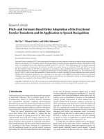
Figure 1. The spectrum of the operator T for different
values of the parameters a and b.

Theorem 3.3. The spectrum of the operator T is given by
{
(3
(1
( 1 3i ) }
i)
i)
σ(T ) = a +
−
b, a −
+
b, a −
−
b
2 2
2 2
2
2
(see Figure 1).
Proof. For any λ ∈ C, we have
[
]
[
]
b
3
t3 − 3a + (1 + i) t2 + 3a2 + ab(1 + i) + ib2 t
2
2
]

[
3
5
1 2
2
3
+ − a − a b(1 + i) − iab − b3 (1 − i)
2 [
2
4
(
)
b
= (t − λ) t2 + λ − 3a − (1 + i) t
2
]
(
b
3 2)
2
2
+ PT (λ).
+ λ − 3aλ − (1 + i) + 3a + ab(1 + i) + ib
2
2


20

L. P. Castro, R. C. Guerra, and N. M.Tuan

Suppose that
λ ̸∈

{
(3
(1
( 1 3i ) }
i)
i)
a+
−
b, a −
+
b, a −
−
b .
2 2
2 2
2
2

This implies that
[
]
[
]
b
3
PT (λ) = λ3 − 3a + (1 + i) λ2 + 3a2 + ab(1 + i) + ib2 λ

2
2
[
]
1 2
3
5 3
3
2
+ − a − a b(1 + i) − iab − b (1 − i) ̸= 0.
2
2
4
Then the operator T − λI is invertible, and its inverse operator is defined by
[
(
)
1
b
−1
(T − λI) = −
T 2 + λ − 3a − (1 + i) T
PT (λ)
2
]
(
b
3 2)
2
2

+ λ − 3aλ − (1 + i) + 3a + ab(1 + i) + ib I .
2
2
So, we have proved that if T − λI is not invertible, then λ ∈ σ(T ).
Conversely, if we choose λ = t1 , we obtain:
][
[
(
(3
i) )
−
b I T 2 + (−2a + b(1 − i))T
T − a+
2 2
(
) ]
ab
b
2
2
+ a −
(1 − 3i) + 2b − (1 + i) I = −PT (λ)I.
2
2
As λ = a + ( 32 − 2i )b, then PT (λ) = 0. So, if T − (a + ( 32 − 2i )b)I is invertible,
then
(
)
(
)

ab
b
T 2 + − 2a + b(1 − i) T + a2 −
(1 − 3i) + 2b2 − (1 + i) I = 0,
2
2
which implies that b = 0 and this is a contradiction. So, T − (a + ( 32 − 2i )b)I
is not invertible.
The same procedure can be repeated for λ = t2 , t3 , in which cases we
obtain the same desired conclusion.
Thanks to the identity (3.3), we obtain three types of eigenfunctions of T ,
represented as follows:
K
∑

ΦI (x) =
|k|=0

αk φk (x), k ∈ C,

K
∑

ΦII (x) =

|k|=1,2

|k|=3

αk φk (x), k ∈ C,

(3.5)

(mod 4)

K
∑

ΦIII (x) =

(3.4)

(mod 4)

(mod 4)

αk φk (x), k ∈ C.

(3.6)


On Integral Operators Generated by the Fourier Transform and a Reflection

21

3.1.2. Parseval type identity.
Theorem 3.4. A Parseval type identity for T is given by
[
]
3

⟨T f, T g⟩L2 (Rn ) = |a|2 + |b|2 ⟨f, g⟩L2 (Rn ) + 2ℜ{ab}⟨f, F g⟩L2 (Rn )
2 }
{
+ ℜ b(1 − i)a ⟨f, W g⟩L2 (Rn ) + |b|2 ⟨f, F −1 g⟩L2 (Rn ) , (3.7)
for any f, g ∈ L2 (Rn ).
Proof. For any f, g ∈ L2 (Rn ), it is straightforward to verify the following
identities:
⟨W f, W g⟩L2 (Rn ) = ⟨f, g⟩L2 (Rn ) ,

(3.8)

⟨f, W g⟩L2 (Rn ) = ⟨W f, g⟩L2 (Rn ) .

(3.9)

If we have in mind (3.8)–(3.9) and as well that for any f, g ∈ L2 (Rn ):
⟨W f, F g⟩L2 (Rn ) = ⟨f, F −1 g⟩L2 (Rn ) ,
⟨F f, W g⟩L2 (Rn ) = ⟨f, F −1 g⟩L2 (Rn ) ,
⟨F f, F g⟩L2 (Rn ) = ⟨f, g⟩L2 (Rn ) ,

(3.10)

⟨F f, g⟩L2 (Rn ) = ⟨f, F g⟩L2 (Rn ) ,
then (3.7) directly appears by using (1.1).
3.1.3. Integral equations generated by T . Now we will consider the operator
equation, generated by the operator T (on L2 (Rn )), of the following form
mφ + nT φ + pT 2 φ = f,

(3.11)

where m, n, p ∈ C are given, |m| + |n| + |p| ̸= 0, and f is predetermined.
As we proved previously, the polynomial PT (t) has the single roots t1 =
a+( 23 − 2i )b, t2 = a−( 12 + 2i )b and t3 = a−( 12 − 3i
2 )b. The projectors induced
by T , in the sense of the Lagrange interpolation formula, are given by
(T − t2 I)(T − t3 I)
T 2 − (t2 + t3 )T + t2 t3
=
,
(t1 − t2 )(t1 − t3 )
(t1 − t2 )(t1 − t3 )
T 2 − (t1 + t3 )T + t1 t3
(T − t1 I)(T − t3 I)
=
,
P2 =
(t2 − t1 )(t2 − t3 )
(t2 − t1 )(t2 − t3 )
(T − t1 I)(T − t2 I)
T 2 − (t1 + t2 )T + t1 t2
P3 =
=
.
(t3 − t1 )(t3 − t2 )
(t3 − t1 )(t3 − t2 )

P1 =

(3.12)
(3.13)

(3.14)

Then we have
Pj Pk = δjk Pk ,

T ℓ = tℓ1 P1 + tℓ2 P2 + tℓ3 P3 ,

(3.15)

for any j, k = 1, 2, 3, and ℓ = 0, 1, 2. The equation (3.11) is equivalent to
the equation
a1 P1 φ + a2 P2 φ + a3 P3 φ = f,
(3.16)
where aj = m + ntj + pt2j , j = 1, 2, 3.


22

L. P. Castro, R. C. Guerra, and N. M.Tuan

Theorem 3.5.
(i) The equation (3.11) has a unique solution for every f if and only if
a1 a2 a3 ̸= 0. In this case, the solution of (3.11) is given by
−1
−1
φ = a−1
1 P1 f + a2 P2 f + a3 P3 f.

(3.17)

(ii) If aj = 0, for some j = 1, 2, 3, then the equation (3.11) has a
solution if and only if Pj f = 0. If this condition is satisfied, then
the equation (3.11) has an infinite number of solutions given by
(∑ )
∑
φ=
a−1
Pj .
(3.18)
j Pj f + z, where z ∈ ker
j≤3
aj ̸=0

j≤3
aj ̸=0

Proof. Suppose that the equation (3.11) has a solution φ ∈ L2 (Rn ). Applying Pj to both sides of the equation (3.16), we obtain a system of three
equations:
aj Pj φ = Pj f, j = 1, 2, 3.
In this way, if a1 a2 a3 ̸= 0, then we have the following system of equations:

−1

P1 φ = a1 P1 f,
(3.19)
P2 φ = a−1
2 P2 f,


P3 φ = a−1

P
f.
3
3
Using the identity
P1 + P2 + P3 = I,
we obtain (3.17). Conversely, we can verify that φ fulfills (3.16).
If a1 a2 a3 = 0, then aj = 0, for some j ∈ {1, 2, 3}. Therefore, it follows
that Pj f = 0. Then, we have
∑
∑
a−1
Pj φ =
j Pj f.
j≤3
aj ̸=0

j≤3
aj ̸=0

Using the fact that Pj Pk = δjk Pk , we get
]
( ∑ )[ ∑
(∑ )
a−1
Pj
Pj φ =
j Pj f
j≤3
aj ̸=0

j≤3
aj ̸=0

or, equivalently,

(∑
j≤3
aj ̸=0

)[
Pj

φ−

∑

j≤3
aj ̸=0

]
a−1
j Pj f = 0.

j≤3
aj ̸=0

Therefore, we can obtain the solution (3.18).
Conversely, we can verify that φ fulfills (3.16). As the Hermite functions
are the eigenfunctions of T , we can say that the cardinality of all functions

φ in (3.18) is infinite.


On Integral Operators Generated by the Fourier Transform and a Reflection

23

3.1.4. Convolution. In this subsection we will focus on obtaining a new
T

convolution ∗ for the operator T . We will perform it for the case b ̸= 0 and
c = 2b (1 − i), although the same procedure can be implemented for other
cases of the parameters.
This means that we are identifying the operations that have a correspondent multiplication property for the operator T as the usual convolution has
T

for the Fourier transform (T f )(T g) = T (f ∗ g).
Theorem 3.6. For the operator T = aI + bF + cW , with a, b, c ∈ C, b ̸= 0
and c = 2b (1 − i), and f, g ∈ L2 (Rn ), we have the following convolution:
[
T
f ∗ g = C A1 f g + A2 (W f )(W g) + A3 (f W g + g W f )
(
)
+ A4 (f F g + g F f ) + A5 (W f )(F −1 g) + (F −1 f )(W g)
(
)
+ A6 (W f )(F g) + (F f )(W g) + A7 (g F −1 f + f F −1 g)
(
)

+ A8 ((F f )(F g)) + A9 (F −1 f )(F −1 g) + A10 (F (f g))
(
)
+ A11 F (f W g) + F (g W f ) + A12 (F −1 (f g))
(
)
(
)
+ A13 F (f F g) + F (g F f ) + A14 F −1 (f F g) + F −1 (g F f )
(
)
+ A15 F ((F f )(W g)) + F ((W f )(F g))
(
)
+ A16 F −1 ((F f )(W g)) + F −1 ((W f )(F g))
]
+ A17 F ((F f )(F g)) + A18 F −1 ((F f )(F g)) ,
(3.20)
where
C=

a3

+ 12
3

a2 b(1

1
+ i) + 32 iab2 +

5
4

b3 (1 − i)

,

a b
ab3
ib4
(1 + i) + ia2 b2 +
(1 + i) +
,
2
4
4
2 2
3
4
3
a b
ab
b
a b
A2 = −
(1 + i) −
(1 − i) +
−
(1 − i),

2
2
2
2
a3 b
a2 b2
ab3
ab3
A3 =
(1 + i) +
(1 + i) +
(1 + i) −
(1 − i),
2
2
2
4
a2 b2
a2 b2
ab3
A4 = a3 b +
(1 + i) + iab3 , A5 = −
(1 − i) −
,
2
2
2
a2 b2
ab3
b4

ab3
b4
A6 =
(1 − i) +
+
(1 + i), A7 = i
−
(1 − i),
2
2
2
2
4
ab3
ab3
b4
A8 = a2 b2 +
(1 + i) + ib4 , A9 = −
(1 − i) −
,
2
2
2
4
2 2
b
a b
(1 + i) −
(1 + i),
A10 = −a3 b −

2
2
a2 b2
ab3
A11 = −
(1 − i) −
− iab3 ,
2
2
A1 = a4 +


24

L. P. Castro, R. C. Guerra, and N. M.Tuan

A12 = i

ab3
b4
−
(1 − i) + a2 b2 (1 − i),
2
4
A14 = ab3 (1 − i),

A15 = −

A13 = −a2 b2 −

ab3
(1 + i),
2

ab3
b4
(1 − i) −
,
2
2

b4
(1 + i), A18 = b4 (1 − i).
2
Proof. Using the definition of T and a direct (but long) computation, we
obtain the equivalence between (3.20) and
A16 = −ib4 ,

A17 = −ab3 −

1
+
+ i) + 23 iab2 + 54 b3 (1 − i)
[
(
)
(
) ][
]
b

3
× T 2 − 3a + (1 + i) T + 3a2 + ab(1 + i) + ib2 I (T f )(T g) .
2
2
T

f ∗g=

a3

1
2

a2 b(1

Thus, having in mind (3.2), we identify the last identity with
[
]
T
f ∗ g = T −1 (T f )(T g) ,
which is equivalent to

( T )
(T f )(T g) = T f ∗ g ,

as desired.
3.2. Case b ̸= 0 and c ̸= ± 2b (1 ± i). In the case of the operator T :=
aI + bF + cW , a, b, c ∈ C, b ̸= 0 and c ̸= ± 2b (1 ± i), whose characteristic
polynomial is
PT (t) = t4 − 4at3 + (6a2 − 2c2 )t2 + (−4a3 − 4b2 c + 4ac2 )t

+ (a2 − c2 )2 + b2 (4ac − b2 ),
we have the following properties.
3.2.1. Invertibility and spectrum.
Theorem 3.7. T is an invertible operator if and only if
a + c + b ̸= 0,

a − c − ib ̸= 0,

a + c − b ̸= 0,

a − c + ib ̸= 0.

(3.21)

In this case, the inverse operator is defined by the formula
T −1 = −

(a2
[

−

c2 )2

1
+ b2 (4ac − b2 )

]
× T 3 − 4aT 2 + (6a2 − 2c2 )T − (−4a3 − 4b2 c + 4ac2 )I . (3.22)
Proof. Suppose that the operator T is

ctions φk , we have:

(a + c + b)φk (x)



(a − c − ib)φ (x)
k
(T φk )(x) =

(a
+
c
−
b)φ
k (x)



(a − c + ib)φk (x)

invertible. Using the Hermite funif
if
if
if

|k| ≡ 0
|k| ≡ 1
|k| ≡ 2
|k| ≡ 3

(mod
(mod
(mod
(mod

4),
4),
4),
4).

(3.23)


On Integral Operators Generated by the Fourier Transform and a Reflection

25

Therefore,
• for |k| ≡ 0 (mod 4), (T φk )(x) = (a + b + c)φk (x), which implies
that a + c + b ̸= 0;
• for |k| ≡ 1 (mod 4), (T φk )(x) = (a − ib − c)φk (x), which implies
that a − c − ib ̸= 0;
• for |k| ≡ 2 (mod 4), (T φk )(x) = (a − b + c)φk (x), which implies
that a + c − b ̸= 0;
• for |k| ≡ 3 (mod 4), (T φk )(x) = (a + ib − c)φk (x), which implies
that a − c + ib ̸= 0.
Conversely, suppose that (3.21) holds. So,
(a2 − c2 )2 + b2 (4ac − b2 ) ̸= 0.
Hence, it is easy to verify that the operator defined in (3.22) is the inverse

of the operator T .
Remark 3.8.
(1) The characteristic roots of the polynomial PT (t) are
t1 = a + c + b,

t2 = a − c − ib,

t3 = a + c − b,

t4 = a − c + ib.

(2) T is not a unitary operator, unless a = 0, b = eiβ , c = 0, β ∈ R,
(which is the operator T = bF , with b ∈ C \ {0}) or a = eiα , b = 0,
c = 0 or a = 0, b = 0, c = eiγ , α, φ ∈ R, which are not under the
conditions here considered for this operator.
Theorem 3.9. The spectrum of the operator T is defined by
{
}
σ(T ) = a + c + b, a − c − ib, a + c − b, a − c + ib .
Proof. For any λ ∈ C, we have
[
]
t4 −4at3 +(6a2 −2c2 )t2 + − 4a3 −4b2 c+4ac2 t+(a2 −c2 )2 +b2 (4ac−b2 )
[
= (t − λ) t3 + (λ − 4a)t2 + (λ2 − 4aλ + 6a2 − 2c2 )t
(
)]
+ λ3 − 4aλ2 + (6a2 − 2c2 )λ − 4a3 − 4b2 c + 4ac2 + PT (λ).
If λ ̸∈ {a + c + b, a − c − ib, a + c − b, a − c + ib}, then
PT (λ) = λ4 − 4aλ3 + (6a2 − 2c2 )λ2

+ [−4a3 − 4b2 c + 4ac2 ]λ + (a2 − c2 )2 + b2 (4ac − b2 ) ̸= 0.
In this way, the operator T − λI is invertible, and its inverse operator is
defined by the following formula:
1 [ 3
T + (λ − 4a)T 2 + (λ2 − 4aλ + 6a2 − 2c2 )T
(T − λI)−1 = −
PT (λ)
(
) ]
+ λ3 − 4aλ2 + (6a2 − 2c2 )λ − 4a3 − 4b2 c + 4ac2 I .


26

L. P. Castro, R. C. Guerra, and N. M.Tuan

In this way, we have proved that if T − λI is not invertible, then λ ∈ σ(T ).
Conversely, if we choose λ = t1 , we obtain:
(
)[
T − (a + c + b)I T 3 + (−3a + b + c)T 2
+ (3a2 − 2ab + b2 − 2ac + 2bc − c2 )T + (−a3 + a2 b − ab2 + b3 + 4ac
]
+ a2 c − 2abc − b2 c − 3ac2 + bc2 − c3 )I = −PT (λ)I.
As λ = a + c + b, PT (λ) = 0. So, if T − (a + c + b)I is invertible, then
T 3 + (−3a + b + c)T 2 + (3a2 − 2ab + b2 − 2ac + 2bc − c2 )T
+ (−a3 + a2 b − ab2 + b3 + 4ac + a2 c − 2abc − b2 c − 3ac2 + bc2 − c3 )I = 0,
which implies that a = 0 and b = 0 or that b = 0 and c = 0, which
is not under the conditions imposed for this operator. So, we reach to a
contradiction. Hence, T − (a − c − b(1 + i))I is not invertible.

Arguing in the same way for λ = t2 , t3 , t4 , we obtain a very similar
conclusion.
Thanks to the identity (3.23), we obtain four types of eigenfunctions of T ,
represented as follows:
ΦI (x) =

K
∑

αk φk (x), k ∈ C,

(3.24)

αk φk (x), k ∈ C,

(3.25)

αk φk (x), k ∈ C,

(3.26)

αk φk (x), k ∈ C.

(3.27)

|k|≡0 (mod 4)

ΦII (x) =

K

∑
|k|≡1 (mod 4)

ΦIII (x) =

K
∑
|k|≡2 (mod 4)

ΦIV (x) =

K
∑
|k|≡3 (mod 4)

3.2.2. Parseval type identity. In the present case, a Parseval type identity
takes the following form.
Theorem 3.10. In the present case, a Parseval type identity for T is
given by
[
]
⟨T f, T g⟩L2 (Rn ) = |a|2 + |b|2 + |c|2 ⟨f, g⟩L2 (Rn ) + 2ℜ{ab}⟨f, F g⟩L2 (Rn )
+ 2ℜ{ac}⟨f, W g⟩L2 (Rn ) + 2ℜ{bc}⟨f, F −1 g⟩L2 (Rn )

(3.28)

for any f, g ∈ L2 (Rn ).
Proof. The formula (3.28) is a direct consequence of (1.1), (3.8), (3.9) and
(3.10).

On Integral Operators Generated by the Fourier Transform and a Reflection

27

3.2.3. Integral equations generated by T . As before, we will now consider in
the present case the following operator equation generated by the operator
T , on L2 (Rn ),
mφ + nT φ + pT 2 φ = f,

(3.29)

where m, n, p ∈ C are given, |m| + |n| + |p| ̸= 0, and f is predetermined.
The polynomial PT (t) has the single roots: t1 = a + c + b, t2 = a − c − ib,
t3 = a + c − b, t4 = a − c + ib. Using the Lagrange interpolation structure,
we construct the projectors induced by T :
P1 =
=
P2 =
=
P3 =
=
P4 =
=

(T − t2 I)(T − t3 I)(T − t4 I)
(t1 − t2 )(t1 − t3 )(t1 − t4 )
T 3 − (t2 + t3 + t4 )T 2 + (t2 t3 + t2 t4 + t3 t4 )T
(t1 − t2 )(t1 − t3 )(t1 − t4 )
(T − t1 I)(T − t3 I)(T − t4 I)

(t2 − t1 )(t2 − t3 )(t2 − t4 )
T 3 − (t1 + t3 + t4 )T 2 + (t1 t3 + t1 t4 + t3 t4 )T
(t2 − t1 )(t2 − t3 )(t1 − t4 )
(T − t1 I)(T − t2 I)(T − t4 I)
(t3 − t1 )(t3 − t2 )(t3 − t4 )
T 3 − (t1 + t2 + t4 )T 2 + (t1 t2 + t1 t4 + t2 t4 )T
(t3 − t1 )(t3 − t2 )(t3 − t4 )
(T − t1 I)(T − t2 I)(T − t3 I)
(t4 − t1 )(t4 − t2 )(t4 − t3 )
T 3 − (t1 + t2 + t3 )T 2 + (t1 t2 + t1 t3 + t2 t3 )T
(t4 − t1 )(t4 − t2 )(t4 − t3 )

− t2 t3 t4 I

− t1 t3 t4 I

− t1 t2 t4 I

− t1 t2 t3 I

,

(3.30)

,

(3.31)

,

(3.32)

.

(3.33)

Then, we have
Pj Pk = δjk Pk ; T ℓ = tℓ1 P1 + tℓ2 P2 + tℓ3 P3 + tℓ4 P4 ,

(3.34)

for any j, k = 1, 2, 3, 4, and ℓ = 0, 1, 2. The equation (3.29) is equivalent to
the equation
a1 P1 φ + a2 P2 φ + a3 P3 φ + a4 P4 φ = f,

(3.35)

where aj = m + ntj + pt2j , j = 1, 2, 3, 4.
Theorem 3.11.
(i) Equation (3.29) has a unique solution for every f if and only if
a1 a2 a3 a4 ̸= 0. In this case, the solution is given by
−1
−1
−1
φ = a−1
1 P1 f + a2 P2 f + a3 P3 f + a4 P4 f.

(3.36)

(ii) If aj = 0, for some j = 1, 2, 3, 4, then the equation (3.11) has a

solution if and only if Pj f = 0. If we have this, then the equation


28

L. P. Castro, R. C. Guerra, and N. M.Tuan

(3.11) has an infinite number of solutions given by
(∑ )
∑
φ=
a−1
Pj .
j Pj f + z, where z ∈ ker
j≤4
aj ̸=0

(3.37)

j≤4
aj ̸=0

Proof. Suppose that the equation (3.29) has a solution φ ∈ L2 (Rn ). Applying Pj to both sides of the equation (3.35), we obtain the system of four
equations: aj Pj φ = Pj f, j = 1, 2, 3, 4.
If a1 a2 a3 a4 ̸= 0, then we have the following system of equations:

P1 φ = a−1

1 P1 f,



P φ = a−1 P f,
2
2
2
(3.38)
P3 φ = a−1
P
3 f,

3


P4 φ = a−1
4 P4 f.
Using the identity
P1 + P2 + P3 + P4 = I,
we obtain (3.36). Conversely, we can verify that φ fulfills (3.35).
If a1 a2 a3 a4 = 0, then aj = 0 for some j ∈ {1, 2, 3, 4}. It follows that
Pj f = 0. Then, we have
∑
∑
a−1
Pj φ =
j Pj f.
j≤4
aj ̸=0

j≤4
aj ̸=0

Using Pj Pk = δjk Pk , we obtain
]
( ∑ )[ ∑
(∑ )
a−1
Pj
Pj φ =
j Pj f .
j≤4
aj ̸=0

Equivalently,

(∑
j≤4
aj ̸=0

j≤4
aj ̸=0

j≤4
aj ̸=0

)[
Pj

φ−

∑

]
a−1
j Pj f = 0.

j≤4
aj ̸=0

So, we obtain the solution (3.37).
Conversely, we can verify that φ fulfills (3.35). As the Hermite functions
are the eigenfunctions of T , we can say that the cardinality of all functions
φ in (3.37) is infinite.
T

3.2.4. Convolution. In this subsection we will present a new convolution ∗
for the operator T . We will perform it for the case b ̸= 0 and c ̸= ± 2b (1 ± i).
This means that we are identifying the operations that have a correspondent
multiplication property for the operator T as the usual convolution has for
T

the Fourier transform (T f )(T g) = T (f ∗ g).


On Integral Operators Generated by the Fourier Transform and a Reflection

29

Theorem 3.12. For the operator T = aI + bF + cW , with a, b, c ∈ C, b ̸= 0
and c ̸= ± 2b (1 ± i), and f, g ∈ L2 (Rn ), we have the following convolution:
[

T
f ∗ g = C A1 f g + A2 (W f )(W g) + A3 (f W g + g W f )
(
)
+ A4 (f F g + g F f ) + A5 (W f )(F −1 g) + (F −1 f )(W g)
(
)
+ A6 (W f )(F g) + (F f )(W g) + A7 (g F −1 f + f F −1 g)
(
)
+ A8 ((F f )(F g)) + A9 (F −1 f )(F −1 g)
(
)
+ A10 (F (f g)) + A11 F (f W g) + F (g W f ) + A12 (F −1 (f g))
(
)
(
)
+ A13 F (f F g) + F (g F f ) + A14 F −1 (f F g) + F −1 (g F f )
( (
)
(
))
+ A15 F (F f )(W g) + F (W f )(F g)
(
(
)
(
))
+ A16 F −1 (F f )(W g) + F −1 (W f )(F g)

(
)
(
)]
+ A17 F (F f )(F g) + A18 F −1 (F f )(F g) ,
(3.39)
where
C=−

1
,
(a2 − c2 )2 + b2 (4ac − b2 )

A1 = 7a5 − 7a3 c2 + 7a2 b2 c − ab2 c2 + a2 c3 − c5 ,
A2 = 7a3 c2 − 7ac4 + 7b2 c3 − a3 b2 + a4 c − a2 c3 ,
A3 = 7a4 c − 7a2 c3 + 7ab2 c2 − a2 b2 c + a3 c2 − ac4 ,
A4 = 7a4 b − 7a2 bc2 + 7ab3 c,

A5 = −a2 b3 + a3 bc − abc3 ,

A6 = 7a3 bc − 7abc3 + 7b3 c2 ,

A7 = −ab3 c + a2 bc2 − bc4 ,

A8 = 7a3 b2 − 7ab2 c2 + 7b4 c,

A9 = −ab4 + a2 b2 c − b2 c3 ,

A10 = a4 b + a2 bc2 + b3 c − 2abc3 ,
A11 = a3 bc + abc3 + ab3 c − 2a2 bc2 ,

A12 = a2 bc2 + bc4 + a2 b3 − 2a3 bc,
A14 = ab4 − 2a2 b2 c,
A16 = b4 c − 2ab2 c2 ,

A13 = a3 b2 + ab2 c2 ,

A15 = a2 b2 c + b2 c3 ,

A17 = a2 b3 + b3 c2 ,

A18 = b5 − 2ab3 c.

Proof. Using the definition of T , by computation we obtain the equivalence
between (3.39) and
1
T
f ∗g=− 2
2
2
(a − c ) + b2 (4ac − b2 )
[
][
]
× T 3 − 4aT 2 + (6a2 − 2c2 )T − (−4a3 − 4b2 c + 4ac2 )I (T f )(T g) .
Consequently, having in mind (3.22), we identify the last identity with
[
]
T
f ∗ g = T −1 (T f )(T g) ,

30

which is equivalent to

L. P. Castro, R. C. Guerra, and N. M.Tuan

( T )
(T f )(T g) = T f ∗ g ,

as desired.
Acknowledgments
This work was supported in part by the Center for Research and Development in Mathematics and Applications, through the Portuguese Foundation
for Science and Technology (“FCT–Fundação para a Ciência e a Tecnologia”), within project UID/MAT/04106/2013.
N. M. Tuan was partially supported by the Viet Nam National Foundation for Science and Technology Development (NAFOSTED).
References
1. P. K Anh, N. M. Tuan, and P. D. Tuan, The finite Hartley new convolutions and
solvability of the integral equations with Toeplitz plus Hankel kernels. J. Math. Anal.
Appl. 397 (2013), No. 2, 537–549.
2. R. N. Bracewell, The Fourier transform and its applications. Third edition.
McGraw-Hill Series in Electrical Engineering. Circuits and Systems. McGraw-Hill
Book Co., New York, 1986.
3. R. N. Bracewell, The Hartley transform. Oxford Science Publications. Oxford Engineering Science Series, 19. The Clarendon Press, Oxford University Press, New
York, 1986.
4. R. N. Bracewell, Aspects of the Hartley transform. Proceedings of the IEEE
82(1994), No. 3, 381–387.
5. G. Bogveradze and L. P. Castro, Wiener–Hopf plus Hankel operators on the
real line with unitary and sectorial symbols. Operator theory, operator algebras, and
applications, 77–85, Contemp. Math., 414, Amer. Math. Soc., Providence, RI, 2006.
6. G. Bogveradze and L. P. Castro, Toeplitz plus Hankel operators with infinite

index. Integral Equations Operator Theory 62 (2008), No. 1, 43–63.
7. L. P. Castro, Regularity of convolution type operators with PC symbols in Bessel
potential spaces over two finite intervals. Math. Nachr. 261/262 (2003), 23–36.
8. L. P. Castro and D. Kapanadze, Dirichlet–Neumann-impedance boundary value
problems arising in rectangular wedge diffraction problems. Proc. Amer. Math. Soc.
136 (2008), No. 6, 2113–2123.
9. L. P. Castro and D. Kapanadze, Exterior wedge diffraction problems with Dirichlet, Neumann and impedance boundary conditions. Acta Appl. Math. 110 (2010),
No. 1, 289–311.
10. L. P. Castro and D. Kapanadze, Wave diffraction by wedges having arbitrary
aperture angle. J. Math. Anal. Appl. 421 (2015), No. 2, 1295–1314.
11. L. P. Castro and A. S. Silva, Invertibility of matrix Wiener–Hopf plus Hankel
operators with symbols producing a positive numerical range. Z. Anal. Anwend. 28
(2009), No. 1, 119–127.
12. L. P. Castro and E. M. Rojas, Explicit solutions of Cauchy singular integral equations with weighted Carleman shift. J. Math. Anal. Appl. 371 (2010), No. 1, 128–133.
13. L. P. Castro and E. M. Rojas, On the solvability of singular integral equations
with reflection on the unit circle. Integral Equations Operator Theory 70 (2011), No.
1, 63–99.
14. L. P. Castro and E. M. Rojas, Bounds for the kernel dimension of singular integral
operators with Carleman shift. Application of mathematics in technical and natural
sciences, 68–76, AIP Conf. Proc., 1301, Amer. Inst. Phys., Melville, NY, 2010.


On Integral Operators Generated by the Fourier Transform and a Reflection

31

15. G. B. Folland and A. Sitaram, The uncertainty principle: a mathematical survey.
J. Fourier Anal. Appl. 3 (1997), No. 3, 207–238.
16. H.-J. Glaeske and V. K. Tuấn, Mapping properties and composition structure of
multidimensional integral transforms. Math. Nachr. 152 (1991), 179–190.

17. B. T. Giang, N. V. Mau, and N. M. Tuan, Operational properties of two integral transforms of Fourier type and their convolutions. Integral Equations Operator
Theory 65 (2009), No. 3, 363–386.
18. K. B. Howell, Fourier Transforms. The Transforms and Applications Handbook
(A. D. Poularikas, ed.). The Electrical Engineering Handbook Series (Third Ed.),
CRC Press with IEEE Press, Boca–Raton–London–New York, 2010.
19. G. S. Litvinchuk, Solvability theory of boundary value problems and singular integral equations with shift. Mathematics and its Applications, 523. Kluwer Academic
Publishers, Dordrecht, 2000.
20. V. Namias, The fractional order Fourier transform and its application to quantum
mechanics. J. Inst. Math. Appl. 25 (1980), No. 3, 241–265.
21. A. P. Nolasco and L. P. Castro, A Duduchava–Saginashvili’s type theory for
Wiener-Hopf plus Hankel operators. J. Math. Anal. Appl. 331 (2007), No. 1, 329–341.
22. D. H. Phong and E. M. Stein, Models of degenerate Fourier integral operators and
Radon transforms. Ann. of Math. (2) 140 (1994), No. 3, 703–722.
23. E. C. Titchmarsh, Introduction to the theory of Fourier integrals. Third edition.
Chelsea Publishing Co., New York, 1986.
24. N. M. Tuan and N. T. T. Huyen, The solvability and explicit solutions of two
integral equations via generalized convolutions. J. Math. Anal. Appl. 369 (2010),
No. 2, 712–718.
25. N. M. Tuan and N. T. T. Huyen, Applications of generalized convolutions associated
with the Fourier and Hartley transforms. J. Integral Equations Appl. 24 (2012), No.
1, 111–130.
26. N. M. Tuan and N. T. T. Huyen, The Hermite functions related to infinite series
of generalized convolutions and applications. Complex Anal. Oper. Theory 6 (2012),
No. 1, 219–236.

(Received 31.08.2015)
Authors’ addresses:
L. P. Castro, R. C. Guerra
CIDMA – Center for Research and Development in Mathematics and
Applications, Department of Mathematics, University of Aveiro, 3810-193

Aveiro, Portugal.
E-mail: ;
N. M. Tuan
Department of Mathematics, College of Education, Viet Nam National
University, G7 Build., 144 Xuan Thuy Rd., Cau Giay Dist., Hanoi, Vietnam.
E-mail: