DSpace at VNU: Enhancing clustering quality of geo-demographic analysis using context fuzzy clustering type-2 and particle swarm optimization

G Model

ARTICLE IN PRESS

ASOC-2296; No. of Pages 19

Applied Soft Computing xxx (2014) xxx–xxx

Contents lists available at ScienceDirect

Applied Soft Computing
journal homepage: www.elsevier.com/locate/asoc

Enhancing clustering quality of geo-demographic analysis using
context fuzzy clustering type-2 and particle swarm optimization
Le Hoang Son ∗
VNU University of Science, Vietnam National University, Viet Nam

a r t i c l e

i n f o

Article history:
Received in revised form 14 February 2014
Available online xxx
Keywords:
Context clustering
Fuzzy clustering type-2
Geo-demographic analysis
Heuristic algorithms
Particle swarm optimization

a b s t r a c t
Geo-Demographic Analysis, which is one of the most interesting inter-disciplinary research topics
between Geographic Information Systems and Data Mining, plays a very important role in policies decision, population migration and services distribution. Among some soft computing methods used for this
problem, clustering is the most popular one because it has many advantages in comparison with the
rests such as the fast processing time, the quality of results and the used memory space. Nonetheless, the
state-of-the-art clustering algorithm namely FGWC has low clustering quality since it was constructed on
the basis of traditional fuzzy sets. In this paper, we will present a novel interval type-2 fuzzy clustering
algorithm deployed in an extension of the traditional fuzzy sets namely Interval Type-2 Fuzzy Sets to
enhance the clustering quality of FGWC. Some additional techniques such as the interval context variable, Particle Swarm Optimization and the parallel computing are attached to speed up the algorithm. The
experimental evaluation through various case studies shows that the proposed method obtains better
clustering quality than some best-known ones.
© 2014 Elsevier B.V. All rights reserved.

Introduction
Geo-Demographic Analysis (GDA), which was defined as “the
analysis of spatially referenced geo-demographic and lifestyle
data”[33], is one of the most interesting inter-disciplinary research
topics between Geographic Information Systems and Data Mining,
and is widely used in the public and private sectors for the planning
and provision of products and services. There are various examples
showing the needs of GDA in practical applications. Shelton et al.
[34] performed a geo-demographic classification for mortality patterns in Britain and found the main causes of deaths in England
and Wales from 1981 to 2000 associated with geographical locations in a map so that they could assist decision makers in better
understanding the distribution of major causes. Michael [23] conducted a GDA analysis to gather community attitudes on the future
growth of Werri Beach and Gerringong, NSW (Nelson), Australia
focusing primarily on what actions Council should take to manage
population growth within existing neighborhoods. Páez et al. [29]
presented a geo-demographic framework using data from Montreal, Canada to identify potential commercial partnerships that
could exploit the characteristics of smart cards. Campbell et al. [8]

∗ Correspondence to: 334 Nguyen Trai, Thanh Xuan, Hanoi 010000, Viet Nam.
Tel.: +84 904171284; fax: +84 0438623938.
E-mail addresses: ,

provided a detailed GDA of over 37,000 gifted and talented students
admitted to the National Academy for Gifted and Talented Youth
in England in 2003/2005 and showed that National Academy had
nonetheless reached significant numbers of students in the poorest
areas, something over 3000 students, and 8% of students identified
as gifted and talented at this stage. Day et al. [11] took a survey
that determined clusters of nations grouped by health outcomes by
comparing life expectancy and a range of health system indicators
within and between each cluster in order to provide sensible groupings for international comparisons. Some other typical applications
of GDA such as the spatial and socio-economic determinants of
tuberculosis, urban green space accessibility for different ethnic
and religious groups, children disorders investigation, etc. could be
referenced in the articles [1,6,9,32,36,37].
In order to perform GDA, some soft computing methods
are often used such as Principal Component Analysis (PCA), SelfOrganizing Maps (SOM) and clustering. Walford [41] described a
method using PCA to study the spatial distribution of the 1991 census data scores. However, results of PCA depend on the scaling of
the variables, and its applicability is limited by certain assumptions made in the derivation. Loureiro et al. [21] introduced the
use of SOM as an adequate tool for GDA. Based on the variations in
edge length in a path between two units on the SOM, the authors
presented a new way of calculating fuzzy memberships of fuzzy
clustering method. However, it requires a lot of memory spaces to
store all neurons and weights; what is more the speed of training

/>1568-4946/© 2014 Elsevier B.V. All rights reserved.

Please cite this article in press as: L.H. Son, Enhancing clustering quality of geo-demographic analysis using context fuzzy clustering
type-2 and particle swarm optimization, Appl. Soft Comput. J. (2014), />

G Model

ARTICLE IN PRESS

ASOC-2296; No. of Pages 19

L.H. Son / Applied Soft Computing xxx (2014) xxx–xxx

2

phase is quite slow. Because of some limitations in those methods,
clustering is often used instead because it has many advantages
in comparison with the rests such as the fast processing time, the
quality of results and the used memory space. Our previous work
in [36] made an overview about some clustering methods for GDA
such as Fuzzy C-Mean (FCM) [3], the agglomerative hierarchical
clustering [11], Neighborhood Effects (NE) [13], K-Means clustering
[20] and Fuzzy Geographically Weighted Clustering (FGWC) [24].
Among them, FGWC was considered the most favorite algorithm
and was used in most of research articles about GDA applications.

u k = ˛ × uk + ˇ ×

1
×
A

c

wkj × uj

(1)

j=1

˛+ˇ =1
wkj =

(2)

(popk × popj )b
a
dkj

(3)

FGWC calculates the influence of one area upon another by Eqs.
(1)–(3) where uk (uk ) is the new (old) cluster membership of the
area k. Two parameters ˛ and ˇ are the scaling variables. popk ,
popj are the populations of areas k and j, respectively. The number dkj is the distance between k and j. Two numbers a and b are
user definable parameters. A is a factor to scale the “sum” term
and is calculated across all clusters, ensuring that the sum of the
memberships for a given area for all clusters is equal to one.
Although FGWC is the most popular clustering algorithm for
GDA, it still contains some limitations such as the speed of computing and the clustering quality. One of our previous works in [35]
presented a method so-called CFGWC to accelerate the speed of
computing of FGWC by attaching the context variable terms. Other

works in [36,37] have showed some preliminary results in improving the clustering quality of FGWC through intuitionistic fuzzy sets
and geographical spatial effects. Thus, our focus in this work is to
continue with the clustering quality problem of FGWC. Based upon
the observation that FGWC was constructed on the basis of the traditional fuzzy sets, which contain some limitations in membership
degrees as pointed out by Mendel [25], this fosters us to improve
FGWC in an extension of the traditional fuzzy sets to enhance the
clustering quality of the algorithm. Now, let us explain why clustering algorithms on the traditional fuzzy sets have low clustering
quality.
According to Mendel [25], the traditional fuzzy sets cannot process some exceptional cases where the membership degrees are
not the crisp values but the fuzzy ones instead. For example, the
possibility to get tuberculosis disease of a patient concluded by a
doctor is from 60 to 80 percents after examining all symptoms. Even
if some modern medical machines are provided, the doctor cannot
give an exact number of that possibility. This shows the fact that
crisp membership values cannot model some situations in the real
world and should be replaced with the fuzzy ones. Rhee [30] stated
that using the traditional fuzzy sets often results in bad clustering
quality because their uncertainties such as distance measure, fuzzifier, centers, prototype and initialization of prototype parameters
can create imperfect representations of the pattern sets. For example, in case of pattern sets that contain clusters of different volume
or density, it is possible that patterns staying on the left side of
a cluster may contribute more for the other rather than this cluster so that choosing suitable value for the fuzzifier is difficult. Bad
selection can yield undesirable clustering results for pattern sets
that include noise. Because of those limitations, some preliminary
results of deploying fuzzy clustering methods in an extension of
the traditional fuzzy sets so-called Interval Type-2 Fuzzy Sets (IT2FS)

have been introduced. Mendel [25] described the definition of IT2FS
as follows.
˜=
A

(x, u,

˜ (x, u)
A

= 1)|∀x ∈ A, ∀u ∈ JX ⊆ [0, 1] .

(4)

From Eq. (4), we recognize that IT2FS is a generalization of the
traditional fuzzy sets since IT2FS will return to the traditional fuzzy
sets when there is no uncertainty in the third dimension. Based
upon this definition, some authors introduced several interval type2 fuzzy clustering algorithms such as in the works of Hwang and
Rhee [15] and Rhee [30]. Specifically, Hwang and Rhee [15] presented a type-2 fuzzy clustering algorithm to solve the problem of
choosing distance measures in FCM algorithm, taking the difference
of each type-2 membership function area with the corresponding
type-1 membership value. Rhee [30] presented an improvement
of this algorithm using two different values of fuzzifiers to solve
the uncertainty of fuzzifier in FCM. Some other variants of the
interval type-2 fuzzy clustering algorithms could be referenced in
[2,10,12,14,17,19,22,26,27,31,42].
Motivated by those results, in this article, we will present a novel
interval type-2 fuzzy clustering algorithm so-called Context Fuzzy
Geographically Weighted Clustering on IT2FS or in short CFGWC2 to
enhance the clustering quality of FGWC. The difference of CFGWC2
with those interval type-2 fuzzy clustering algorithms above is two
fold: Firstly, CFGWC2 is specially designed for the GDA problem
that requires the modification of geographical spatial effects to
the algorithm itself; secondly, it is equipped with some additional

techniques to speed up the whole algorithm, namely:
• An interval context variable, which is an extension of the single
context variable of Pedrycz [28], is proposed and used to clarify
the clustering results and accelerate the computing speed.
• In order to avoid bad initialization, which may occur in other
interval type-2 fuzzy clustering algorithms, and to converge
quickly to the (sub-) optima solutions, a meta-heuristic optimization method namely Particle Swarm Optimization – PSO [18] is
used to determine good initial centers for CFGWC2.
• Since context values in the interval context variable can be simultaneously processed in CFGWC2, parallel computing technique is
adapted to CFGWC2 to reduce the computational costs.
What have been listed in those bullets are our contributions in
this paper. The proposed algorithm will be implemented and compared with some relevant methods in term of clustering quality to
verify its efficiency.
The rests of this paper are organized as follows. Section
“The proposed methodology” elaborates the proposed method in
details including those additional techniques one-after-another.
The numerical experiments through various case studies and
discussions are given in Section “Results”. Finally, Section “Conclusions” gives the conclusions and outlines future works of this
article.

The proposed methodology
In the previous section, we have known that CFGWC2 is an
interval type-2 fuzzy clustering algorithm equipped with some
additional techniques such as the interval context variable, PSO
and the parallel computing for the GDA problem. Since those techniques are necessary for the description of CFGWC2, they are firstly
presented in Sections “Using PSO for the determination of initial
centers” and “The interval context”. The CFGWC2 algorithm accompanied with the parallel computing mechanism will be described
in Section “Evaluation by various case studies”.

Please cite this article in press as: L.H. Son, Enhancing clustering quality of geo-demographic analysis using context fuzzy clustering

type-2 and particle swarm optimization, Appl. Soft Comput. J. (2014), />

G Model

ARTICLE IN PRESS

ASOC-2296; No. of Pages 19

L.H. Son / Applied Soft Computing xxx (2014) xxx–xxx

Using PSO for the determination of initial centers

point to the ith cluster, for instance, using the sum operator (18) or
maximum operator (19).

This section mentions the technique that finds good initial centers for clustering algorithms by PSO. The idea of this technique is
to give a preliminary classification of the original pattern set so that
“temporal” cluster results can be used to orient the classification in
the main algorithm. The objective function is shown in Eq. (5), and
its constrains are given in Eqs. (6)–(7):
N

C

J=

Xk − Vj

2

→ min .

(5)

k=1 j=1

min
j = 1, C

Vi − Vj

>

max

Xs − Vi

s=1,POP(i)

j=
/ i
Xs ∈ Cluster(i)

(6)

i = 1, C
Cluster(i) ≤ ε1 where POP(i) = 1 and i = 1, C

(7)

Constrain (6) requires that all clusters are separated from the
others. Alternatively, the minimal distance from a cluster’s center
to the others is not shorter than the maximal one from this center to
all data points in the cluster. POP(i) is the population or number of
patterns in the cluster Cluster(i). Constrain (7) minimizes the number of outliers in the result. Accordingly, the number of outliers is
not greater than a pre-defined threshold ε1 .
For the problem (5)–(7), we use PSO [18] to determine the (sub) optima solutions with the beginning population being initiated
with P particles. Each particle is a vector z = (z1 , z2 , .., zC ) where
zi (i = 1, C) is a pattern randomly chosen from the original pattern
set. The velocities of zi are set to zeros. Details of the algorithm are
described by the pseudo-code in Table 1.
Notice that Eq. (9) is used solely for the first iteration of
MaxStep PSO. In the next iterations, the centers are calculated from
the previous one. Additionally, the value of MDi in Eq. (10) is set to
zero in case that this cluster has not got any element. The fitness
value of a particle is calculated by Eq. (13) where ( 1 , 2 ) are the
ratio constants. Eqs. (14)–(16) are used to update the velocities and
positions of all particles. In those equations, c1 is the ratio to keep
the velocity intact, c2 is the ratio to change the velocity following
by pBest and c3 shows the influence level of gBest to the velocity.
Since the role of zi (i = 1, C) from the second iteration afterwards
is replaced with center Vi , the domain of random number in Eq.
(14) is set to (−1, 1) in order to ensure the values of the centers
are bounded within the domain of the pattern set. After a number
of iteration steps defined by MaxStep PSO, the solution is getting
better because of the amelioration process after each “flying step”
based on the fitness function. The outputted result V(0) = (V1 , V2 , ..,
VC ) can be found from the particle holding current gBest and is used
as the initial center for CFGWC2.
The interval context

In order to clarify the clustering results and accelerate the computing speed of the clustering algorithms, the context variable
could be used. According to Pedrycz [28], a (single) context variable
in Y ⊂ X is defined through the map below.
A : Y → [0, 1]
yk → fk = A(yk ),

3

(17)

where fk can be understood as the representation for the level of
relation of the kth point to the supposed context fk . There are some
ways to define the relation between fk and the membership of kth

c

uki = fk , k = 1, N,

(18)

maxuki = fk , k = 1, N

(19)

i=1
c

i=1

In our previous work in [35], we defined a context variable to

narrow the original geographical dataset under some conditions of
certain dimensions. The reason to use the term of context for the
clustering algorithm is twofold. Firstly, a context variable is useful
to clarify the results following by users’ purposes. Because only a
subset of the original dataset which has considerable meaning to
the context is invoked, the result focuses on the area that really
has many relevant points. Secondly, it helps improving the speed of
computing. In the traditional clustering method, it not only takes
long time to process the whole data, but also makes the results less
meaning to the considered context. On the contrary, the contextbased clustering methods both accelerate the speed and improve
the semantic. Nevertheless, there are some limitations in definition (17). Firstly, the importance of the kth point to the supposed
context is decided by a value fk . In fact, it is not enough to reflect
a variety of different evaluations of many people to this relation.
In the other words, one can assume that the importance is only 0.3
while other affirms that it should be 0.6. Due to this fact, the use of a
value fk is not enough. Secondly, the old approach excludes the roles
of other data points to the context. It is a misleading assumption
since all characteristics always have relationships either directly
or indirectly with the others. From these limitations, we extend
the use of context by introducing a new term: “the interval context
variable”. An interval context is defined as f = [f1 ,f2 ] where each fi
(i = 1,2) is stated through the map in Eq. (17). For the most important points, the value of f is high, e.g. [0.6,0.8]. Similarly, the value
of f in case of less important points is low, e.g. [0,0.15]. This interval
reflects the “fuzziness” of the context. In the other words, we have
just performed a “fuzzy” step for the considered context. It helps
us overcome the shortcomings of the single context variable and
is suitable for CFGWC2, which works on IT2FS. Details of applying
the interval context variable for CFGWC2 will be presented in the
Section “The CFGWC2 algorithm”.
The CFGWC2 algorithm

We have had a general background of choosing initial centers
by PSO in Section “Using PSO for the determination of initial centers” and the basic definition of the interval context in Section “The
interval context”. Now, we use both of them accompanied with the
parallel computing mechanism in the main activity of the CFGWC2
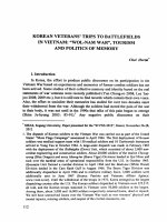
algorithm. Let us see the mechanism of CFGWC2 illustrated by Fig. 1
below.
According to Fig. 1, the parallel computing mechanism of
CFGWC2 requires three machines whose first one (Machine 1)
is responsible for generating initial centers for the remaining
machines. Nevertheless, the centers values of Machine 2 and
Machine 3 are different since the stopping conditions of PSO are not
identical. After (MaxStep PSO/2) iteration steps, the first center V(0)
is outputted and transferred to Machine 2, and the second center
is sent to Machine 3 after (MaxStep PSO) iterations. This guarantees different results in Machine 2 and Machine 3, and is suitable
for the determination of the upper and lower centers and membership degrees of the clustering algorithms on IT2FS, i.e. U(1) , V(1)
(Machine 2) and U(2) , V(2) (Machine 3) in Fig. 1.
In Machine 2 and Machine 3, we send the initial centers V(0) to
a type-2 fuzzy clustering procedure accompanied with the interval

Please cite this article in press as: L.H. Son, Enhancing clustering quality of geo-demographic analysis using context fuzzy clustering
type-2 and particle swarm optimization, Appl. Soft Comput. J. (2014), />

G Model

ARTICLE IN PRESS

ASOC-2296; No. of Pages 19

L.H. Son / Applied Soft Computing xxx (2014) xxx–xxx

4
Table 1
The pseudo-code of PSO procedure.
Input

- The pattern set X whose dimension is r
- The number of elements (clusters) – N(C)
- The number of particles in the beginning population – P
- Maximal number of iteration steps in PSO – MaxStep PSO
- Final center V(0)

Output
Particle Swarm Optimization (PSO)
1:
2:
3:
4:

Initialization
Repeat
For each particle
Assign remaining patterns to its clusters:
Xj ∈ Cluster(i) ⇔

zi − Xj

= min

zk − Xj

|k = 1, C

(8)

5:
6:

Calculate population POP(i)from current clusters
Calculate center Vi and the maximal distance from Vi to cluster’s elements:
(l)

Vi

(l)

=

Xs

/POP(i),

l = 1, r,

MDi =

Xs − Vi

max

i = 1, C

⎧
⎨

Xs∈Cluster(i)

=

s=1,POP(i)

max
s=1,POP(i)

(9)

r

(Xs (l) − Vi (l) )

⎩

l=1

2

⎫
⎬
⎭

,

(10)

Xs ∈ Cluster(i),
7:

Calculate the separated status and the number of outliers:
min
j = 1, C

SEP(z) = Cluster(i)
OUT (z) = Cluster(i)

where

Vi − Vj

/ i
j=

MDi
where POP(i) ≤ 1;

≤ 1;

i = 1, C,

(11)

i = 1, C.

(12)

8:
f (z) =

Compute the fitness value of particles:
1
( 1 /1 + SEP(z)) + (

2 /1

(13)

+ OUT (z))

9:
10:
11:
12:

velocityij = c1 ∗ velocityij + c2 ∗ rand(−1, 1) ∗ (zpBest,j − zij ) + c3 ∗ rand(−1, 1) ∗ (zgBest,j
zij = zij + velocityij ,
c1 + c2 + c3 = 1.
13:
14:

context variable so-called Context-FGWC2 to get the crisp center
V(1) (Machine 2) and V(2) (Machine 3). If the difference between
the initial and crisp centers is smaller than a threshold (Eps) or the

maximal number of iterations (MaxStep) is reached then we stop
the Context-FGWC2 procedure and take the crisp center and membership degree, i.e. U(1) , V(1) (Machine 2) and U(2) , V(2) (Machine 3)
as the final results. Otherwise, we assign V(0) = V(1) in Machine 2 and
V(0) = V(2) in Machine 3 and start a new iteration in Context-FGWC2
until the stopping conditions hold.
Once the upper and lower centers and membership degrees are
calculated, we use a defuzzification method so-called the Partition
Coefficient and Exponential Separation (PCAES) [40] validity index to
obtain the final center and membership degree as below.
V (∗) =

V (1)

if PCAES(V (1) ) ≥ PCAES(V (2) )

V (2)

otherwise

(20)

C

PCAES[j]
j=1

where

⎛
N

ukj

PCAES[j] =
k=1

⎜

2

uM

− exp ⎝

−min{ Vj − Vi
i=
/ j

ˇT

2

}

⎞
⎟
⎠,

(22)

N

u2ki

uM = min

1≤i≤C

(23)

k=1

ˇT =

C
l=1

Vl − V

2

C

(24)

V = (V 1 , V 2 , .., .V r ) where V i (i = 1, r) is calculated as,

This index measures the potential, whether the identified cluster has an ability to be a good cluster or not. It was compared with
other indexes such as Partition Entropy (PE), Partition Coefficient
(PC), Fuzzy Hypervolume (FHV), Xie & Beni, Pal & Bezdek, Modification PC (MPC), Zahid et al., and showed the impressive results, even

in a noisy environment. The definition of PCAES is given below.
PCAES(C) =

Calculate pBest and gBest as in the traditional PSO algorithm [18]
End For
For each particle
Update new velocity and position:
− zij ),
(14)
(15)
(16)
End For
Until MaxStep PSO

(21)

Vi =

C
V
l=1 li

C

.

(25)

PCAES[j] is used to measure the compactness and separation for
cluster j (j = 1, C). They are summed up to calculate PCAES(C) ∈ (− C,

C). The large PCAES(C) value means that each of these C clusters
is compact and separated from other clusters. It is a criterion to
choose the suitable clustering’s output. Depending on which center
is opted, the related membership degree is used as final membership U(*) .
Now, we describe the Context-FGWC2 procedure. Remembering in Section “The interval context” that an interval context was
defined as f = [f1 ,f2 ] so that we could apply fi (i = 1,2) in each machine.

Please cite this article in press as: L.H. Son, Enhancing clustering quality of geo-demographic analysis using context fuzzy clustering
type-2 and particle swarm optimization, Appl. Soft Comput. J. (2014), />

G Model

ARTICLE IN PRESS

ASOC-2296; No. of Pages 19

L.H. Son / Applied Soft Computing xxx (2014) xxx–xxx

5

Table 2
The pseudo-code of Context-FGWC2 procedure.
- Initial center V(0) , the pattern set X, an interval fuzzifier [m1 ,m2 ],
- The number of elements (clusters) – N(C), the dimension of dataset r,
- Geographic parameters ˛, ˇ, a and b, precision ε, MaxStep iteration.
- Final center V(3)

Input

Output

Context-FGWC2

V(3) ← V(0)
Repeat
V(0) ← V(3)

1:
2:
3:

Compute U(x) = U(x), U(x) by (26)–(29)

4:

V(A) ← V(0)
For l = 1, r:
Sort X following by lin ascending order
Find index k0 satisfying (30). Otherwise, k0 ← N − 1
Calculate U(1)(l) , V(1) by (31)–(32)
If V(1) = V(A)

5:
6:
7:
8:
9:
10:

For s = l + 1, r: Ukj (1)(s) ← Ukj (j = 1, C, k = 1, N)
Go to Step 16

Else V(A) ← V(1)
End If
End For
VR ← V(1)
Calculate U(1) by (33)
Repeat from Step 5 to 17 to calculate VL , U(2)
Perform Type-Reduction by (36)
Determine the population of each cluster by (37)
Update U(C) (x) by geo-characteristics in (2), (3) and (38)–(40)
Perform Type-Reduction and compute center V(2) by (41) and (42) to get UGT (x)
V(B) ← V(2)
Repeat from Step 6 to 18 to calculate VR , VL from V(B) and UGT (x)
Perform defuzzification to calculate V(3) by (43)

11:
12:
13:
14:
15:
16:
17:
18:
19:
20:
21:
22:
23:
24:
25:
26:

V (3) − V (0)

Until

≤ ε or MaxStep is reached

Specifically, f1 (f2 ) was used in the Context-FGWC2 procedure
of Machine 2 (3). Because of using different context values and initial centers in those machines, the upper and lower centers and
membership degrees totally reflect the basic principle of IT2FS. The
basic idea of the Context-FGWC2 procedure in Machine 2 is using an
interval of primary membership consisting of the lower and upper
ones calculated from the initial center and updating the interval
by geo-characteristics and context value f1 . The pseudo-code of
Context-FGWC2 is shown in Table 2.
In Step 4 of the Context-FGWC2, the intervals of primary
membership consisting of the upper and lower memberships are
calculated by Eqs. (26)–(29). Notice that in (26)–(27), the sum of
membership degrees in all clusters is equal to f1k where f1k is a
context value of the kth point in the pattern set. Analogously, the
values of the upper and lower memberships are depended by this
context value as shown in (28)–(29).

U(x) =

U(x) =

⎧
⎪
⎪

⎪
⎪
⎪
⎪
⎪
⎨
Ukj =

⎪
⎪
⎪
⎪
⎪
⎪
⎪
⎩

⎧
⎨

C

Ukj ∈ (0, 1)|k = 1, N; j = 1, C;

⎩

Ukj = f1k
j=1

⎧

⎨

C

Ukj ∈ (0, 1)|k = 1, N; j = 1, C;

⎩

Ukj = f1k
j=1

f1k
C

i=1

Xk − Vj

(0)

2/m1 −1

, if

Xk − Vi (0)

C

i=1

Xk − Vj (0)
Xk − Vi (0)

2/m2 −1

,

(26)

⎭

Ukj =

⎪
⎪
⎪
⎪
⎪
⎪
⎪
⎩

(27)

⎭

Xk − Vj

(0)

2/m1 −1

, if

Xk − Vi (0)

i=1

C

Xk − Vj (0)

f1k
C

i=1

f1k
2/m2 −1

,

< 1/C

Xk − Vj (0)
Xk − Vi (0)

(29)
otherwise

Xk − Vi (0)

i=1

After we have the interval of primary membership, the maximum (minimum) center VR (VL ) and the related membership matrix
U(1) (U(2) ) are calculated by the same steps from Step 6 to 17. Specifically, in Step 8 index k0 in the range [1,N − 1] satisfying Eq. (30) will
be selected as a pivot to calculate U(1)(l) in Eq. (31).
Xk0 l ≤

C
v (A)
j=1 jl

(30)

C ≤ X(k0 +1)l
Ukj (1)(l) =

(1)

Vji

Ukj

if k ≤ k0

Ukj

otherwise

,

(j = 1, C,

k = 1, N)

(31)

=

[m1 +m2 /2]
N
Xki
(Ukj (1)(l) )
k=1
,
[m
+m
/2]
N
1
2
(Ukj (1)(l) )
k=1

(j = 1, C,

i = 1, r)

(32)

Next, in Step 10 we check whether V(1) = V(A) or not. If this condition holds, we conclude that the maximum center VR = V(1) and
the related membership matrix U(1) is found in Eq. (33).

≥ 1/C

Xk − Vj (0)
Xk − Vi (0)

(28)
otherwise

f1k
C

Using the average operator of fuzzifier, center V(1) is calculated
below.

⎫
⎬

f1k
C

i=1

f1k

⎫
⎬

⎧
⎪
⎪
⎪
⎪
⎪
⎪
⎪
⎨

U (1) =

r
U (1)(l)
l=1

r

.

(33)

Otherwise, we make another loop with the next feature l in the
pattern set. By the similar process, in Step 18 we can compute the

Please cite this article in press as: L.H. Son, Enhancing clustering quality of geo-demographic analysis using context fuzzy clustering
type-2 and particle swarm optimization, Appl. Soft Comput. J. (2014), />

G Model

ARTICLE IN PRESS

ASOC-2296; No. of Pages 19

L.H. Son / Applied Soft Computing xxx (2014) xxx–xxx

6

(2)

Ukj G = ˛ × Ukj + ˇ ×

1
×
A

C
(2)

wji × Uki

(39)

i=1

G

(1)

Ukj = ˛ × Ukj + ˇ ×

1
×
A

C
(1)

wji × Uki ,

(40)

i=1

(i, j = 1, C, i =
/ j, k = 1, N).
Notice that parameter A in Eqs. (39) and (40) is a factor to scale
the “sum” term and is calculated across all clusters, ensuring that
the sum of the memberships for a given area k for all clusters is
equal to the context value f1k (k = 1, N). Step 22 performs the typereduction for the modified membership degree and calculates new
center V(2) by Eqs. (41) and (42), respectively.
G

Ukj GT =
Vji (2) =

Ukj + Ukj G
2

,

(j = 1, C,

[m1 +m2 /2]
N
(Ukj GT )
Xki
k=1
,
N
GT [m1 +m2 /2]
(Ukj )
k=1

k = 1, N),

(j = 1, C,

(41)

i = 1, r)

(42)

Now, we have modified membership degree UG and crisp center
V(2) . Since we work on IT2FS, V(2) should be an interval containing the minimum and maximum centers VL , VR . This work is done
through Step 23 and 24. In order to verify whether the outputted
centers is the solution or not, Step 25 performs the defuzzification
for the interval center as in Eq. (43) and get crisp one V(3) . This

center is used to check the stopping condition described in Step 26.
V (3) =

Fig. 1. The mechanism of CFGWC2.

minimum center VL and the related membership matrix U(2) where
Eqs. (31) and (33) are replaced with (34) and (35), respectively.
(2)(l)

Ukj

=

U (2) =
U (C) =

Ukj

if k ≤ k0

Ukj

otherwise

,

(j = 1, C,

k = 1, N)

r
U (2)(l)
l=1

(34)

(35)

r
U (1) + U (2)
2

(36)

From these related membership matrices, Step 19 obtains the
membership degree of traditional fuzzy sets (a.k.a. type-1) through
Eq. (36). This process is called the type-reduction and used to calculate the population of each cluster. Step 20 calculates the population
of each cluster by this rule:
(C)

(C)

If Ukj > Uki

and i =
/ j then Xk is assigned to cluster j,

(37)

(k = 1, N; i = 1, C)

Based on the population, Step 21 determines the geographical
weights of all areas by Eq. (3), and the modification of membership
degree following by geo-characteristics is performed through Eqs.
(2), (3) and (38)–(40).
U G (x) = G(U (C) (x)) = Ukj G , Ukj

G

,

(j = 1, C,

k = 1, N)

(38)

VL
VR

if VL − V (0)

≤ VR − V (0)

(43)

otherwise

In order to avoid unstoppable iteration, we limit the maximal
number of iteration steps to MaxStep. If the number of iteration
steps exceeds this threshold, the Context-FGWC2 procedure will

stop immediately. Once the stopping condition holds, we receive
the type-2 membership degree UG and the interval center [VL ,VR ].
The crisp center V(3) and the distribution of pattern set after clustering can be extracted from them. (UG ,V(3) ) are the output of
Context-FGWC2, and the crisp center V(3) is denoted in Fig. 1 as
V(1) (Machine 2) and V(2) (Machine 3).
The works of Context-FGWC2 in Machine 3 is analogous to those
in Machine 2 except the maximal number of iteration steps in
Machine 3 is equal to half of that in Machine 2 (∼MaxStep/2). The
reason for this alteration lies in the synchronization process. Specifically, the results in Machine 2 and 3 are transferred to Machine 1
after completion so that if a machine takes too much time to generate the outputs, it will cause large delayed time of the overall
system. Because the initial center of Machine 3 is somehow better
than that of Machine 2, the convergence may be faster and is not
affected by the number of iteration steps. In practical, the number
of machines can be reduced, for instance the works of the Machine
1 can be assigned to one of two left machines. Because it takes
much time to transfer data between machines, it is better if we can
decrease the waiting time. If so, the number of transferred steps
between machines is reduced by half and the overall processing
time is reduced remarkably.
The advantages of CFGWC2 are fourth-fold: Firstly, it is capable to handle the bad initialization and immature convergence by
the PSO procedure; secondly, the clustering results focus on the
users’ purposes by the interval context; thirdly, the computing
speed of CFGWC2 is ameliorated through the interval context and
the parallel computing mechanism; fourthly, the most important
advantage of CFGWC2 is the high clustering quality in comparison
with some relevant methods since this algorithm was deployed on

Please cite this article in press as: L.H. Son, Enhancing clustering quality of geo-demographic analysis using context fuzzy clustering
type-2 and particle swarm optimization, Appl. Soft Comput. J. (2014), />

G Model
ASOC-2296; No. of Pages 19

ARTICLE IN PRESS
L.H. Son / Applied Soft Computing xxx (2014) xxx–xxx

7

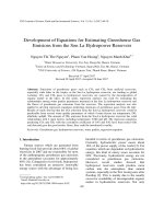
Fig. 2. The two-dimensional distribution of UNO dataset.

IT2FS, which is more general and able to handle the existing limitations of the traditional fuzzy sets. The disadvantage of CFGWC2
could be the computational costs and its complex activities. Nevertheless, by employing some additional techniques we hope that the
disadvantages could be ameliorated, and CFGWC2 achieves good
clustering results.
Results
Experimental environment
This section describes the experimental environment used in
next ones.
• Experimental tools: We have implemented the proposed algorithm (CFGWC2) in addition to these algorithms: NE [13], FGWC
[24] and CFGWC [35] in MPI/C programming language and executed them on a Linux Cluster 1350 with eight computing nodes

of 51.2 GFlops. Each node contains two Intel Xeon dual core
3.2 GHz, 2 GB Ram. The experimental results are taken as the
average values after 10 runs.
• Cluster validity: We use PCAES validity function described in Eqs.
(21)–(25).
• Dataset: We use two kinds of datasets below.
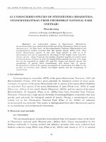
- A real dataset of socio-economic demographic variables from
United Nation Organization (UNO) [39] containing the statistic
about population of 230 countries over ten years (2001–2010).

Missing data were processed by Binning method [16]. The twodimensional distribution is illustrated in Fig. 2.
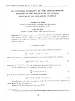
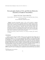
- A benchmark demographic dataset from The University of Edinburgh, Scotland (Fig. 3) including expression levels of 2880
genes taken in 11 different areas [7]. This dataset was used
in many different research papers on gene expression by geographical factors such as in [4,5].
• Objective: We compare the clustering quality of CFGWC2 with
those of other algorithms through PCAES index. Additionally, the

Fig. 3. The two-dimensional distribution of Colon Cancer dataset.

Please cite this article in press as: L.H. Son, Enhancing clustering quality of geo-demographic analysis using context fuzzy clustering
type-2 and particle swarm optimization, Appl. Soft Comput. J. (2014), />

G Model

ARTICLE IN PRESS

ASOC-2296; No. of Pages 19

L.H. Son / Applied Soft Computing xxx (2014) xxx–xxx

8
Table 3
PCAES values of all algorithms in Case 1 on UNO dataset.
C

m = 1.5

m = 2.0

CFGWC2

CFGWC

FGWC

NE

CFGWC2

CFGWC

FGWC

NE

2
3
4
5
6

1091.30832
3508.71041
1026.1004
851.56196
734.85210

11.49441
14.20249
9.66077

13.83029
23.45840

106.87815
102.97090
101.00239
98.86012
105.61367

106.87815
103.08807
101.05883
98.89076
105.11415

730.86493
1764.55205
1882.45315
828.00298
713.06259

15.80779
15.48401
9.60082
20.09243
13.36007

107.95304
104.51216
102.01264

98.70007
106.82538

107.95304
104.62430
102.07279
98.73446
95.32594

C

m = 2.5

2
3
4
5
6

m = 3.0

CFGWC2

CFGWC

FGWC

NE

CFGWC2

CFGWC

FGWC

NE

435.14908
699.52639
758.04253
729.73602
660.41492

15.35085
17.05059
12.13725
13.80425
21.53153

110.80574
112.36477
111.70188
109.59175
107.14039

110.80576
112.46454
111.77472
109.64291
107.19830

222.59648
448.65676
530.12028
544.21607
534.99351

14.84918
18.15664
15.16747
17.33470
18.78905

111.54395
121.39454
123.22859
122.96865
122.06920

111.54397
121.45259
123.30832
123.03807
123.31178

Fig. 4. Average PCAES of algorithms on UNO dataset by fuzzifiers.

evaluation about the computational times of these algorithms is
also mentioned.
Evaluation by various case studies

In this section, we evaluate the proposed algorithm in comparison with the relevant methods by various case studies
about the parameters of algorithms. Main findings are found
below.
Case 1. In this case, some parameters of these algorithms are set
up as below.
- The default geo-characteristics are: a = b = 1, ˛ = 0.7, ˇ = 0.3. These
values determine the geo-modification process stated in Eqs.
(1)–(3). Our previous work [35] suggested using value ˛ ≥ 0.6 in
order to increase the clustering quality.
- We use the default context values in [35] for CFGWC algorithm
below.

where fi =

⎧
⎪
⎨

f = (f1 , f2 , .., fN ),
0

if k = 0

⎪
⎩ rand(0, 1) otherwise
k
2

,

k = imod4,

i = 1, N.
(44)

- In CFGWC2, m2 = 2 × m1 = 2 × m where m is the fuzzifier of NE,
FGWC and CFGWC. The interval context f = f 1 , f 2 where f1 = f
and f2 = 1. A broad interval of fuzzifiers and contexts will create
more distinct results than a narrow one.
- In PSO, MaxStep PSO = 100 and population size is 500. Other
parameters are (c1 , c2 , c3 ) = (0.2, 0.3, 0.5) and ( 1 , 2 ) = (1, 1). As
suggested by Thien et al. [38], these values will make the convergence to the optimum faster.
- Threshold ε and MaxStep of all algorithms are 10−3 and 500,
respectively.

Table 3 describes the PCAES values of all algorithms on UNO
dataset. The experiments are performed following by different values of the number of clusters and fuzzifiers. Results show that
PCAES values of CFGWC2 are the largest among all. This means
that the clustering quality of CFGWC2 is better than those of other
algorithms. In order to comprehend the experimental results, we
illustrate the PCAES values of all algorithms through various cases
of fuzzifiers in Fig. 4. From this figure, we recognize that PCAES
values of CFGWC2 are larger than those of other algorithms.
For example, PCAES of CFGWC2 in Fig. 4 is 13 times greater
than that of FGWC when m = 1.5. These numbers in cases of NE and
CFGWC are 14 and 99 times, respectively. Similarly, when m = 3.0,
PCAES of CFGWC2 is still larger than those of other algorithms, i.e.
3.79 (FGWC), 3.78 (NE) and 27 times (CFGWC). These evidences
confirm that the clustering quality of CFGWC2 is the best among

Please cite this article in press as: L.H. Son, Enhancing clustering quality of geo-demographic analysis using context fuzzy clustering
type-2 and particle swarm optimization, Appl. Soft Comput. J. (2014), />

G Model

ARTICLE IN PRESS

ASOC-2296; No. of Pages 19

L.H. Son / Applied Soft Computing xxx (2014) xxx–xxx
Table 4
The computational time of all algorithms in Case 1 on UNO dataset (s).
C

m = 1.5

m = 2.0

CFGWC2

CFGWC

FGWC

NE

CFGWC2

CFGWC

FGWC

NE

2
3
4
5
6

7.68
14.55
12.94
11.14
20.94

0.04
0.03
0.07
0.07
0.07

0.04
0.09
0.08
0.16
0.24

0.03
0.11

0.12
0.12
0.19

10.165
14.31
12.86
17.49
24.56

0.04
0.04
0.08
0.07
0.11

0.04
0.10
0.11
0.17
0.30

0.04
0.13
0.14
0.14
0.22

C

m = 2.5
CFGWC2

CFGWC

FGWC

NE

CFGWC2

CFGWC

FGWC

NE

5.23
14.98
15.96
17.57
24.82

0.03
0.04
0.09
0.11
0.17

0.04

0.08
0.17
0.19
0.31

0.03
0.15
0.21
0.19
0.36

10.06
15.40
18.06
22.02
24.87

0.04
0.06
0.11
0.27
0.23

0.04
0.09
0.19
0.23
0.36

0.04

0.12
0.17
0.18
0.30

2
3
4
5
6

m = 3.0

all. Nonetheless, PCAES values of CFGWC2 tend to decrease when
the fuzzifier increases. For instance, PCAES values of CFGWC2 from
m = 1.5 to m = 3.0 are 1442, 1183, 656 and 456, respectively. The
average reducing ratio per half of a fuzzifier is 31%. This means that
each time the value of fuzzifier is increased by 0.5, PCAES value of
CFGWC2 is reduced by 31 percents on average. On the other hands,
the average PCAES values of other algorithms seem to be stable
through different values of fuzzifier, i.e. 109 (FGWC), 108 (NE) and
15 (CFGWC). By rough calculation, we can easy find the value of
fuzzifier that makes PCAES value of CFGWC2 is smaller than other
algorithms, i.e. m ≥ 5.0. This fact tells us the truth that CFGWC2
should be used when the fuzzifier is small. As mentioned by Bezdek
et al. [3] when designing FCM algorithm, the authors stated that
the fuzzifier should be from 1.5 to 2.5, ideally m = 2.0, for the sake
of optimal centers found by the algorithm. Thus, we may see that
some cases such as m ≥ 5.0 will never happen in practical applications. However, this finding may be useful for us to choose the
appropriate value of parameters. Is there any change of the order

of algorithms in terms of PCAES values by different values of number of clusters? Following by Table 3, the answer is absolutely no.
For a given number of clusters, PCAES value of CFGWC2 is always
larger than those of algorithms. Indeed, this shows the stability of
the proposed algorithm.
The computational time of all algorithms for exporting the
results in Table 3 is described in Table 4. Clearly, the computational
time of CFGWC2 is longer than those of other algorithms.
When m = 3.0, the average computational time of CFGWC2,
FGWC, NE and CFGWC are 18.1, 0.182, 0.162 and 0.142 s, respectively. Similar results are obtained in m = 2.0 and m = 2.5. As we
may see in the pseudo-code of Context-FGWC2, it requires huge
computation to process the interval membership matrix. By using
some additional techniques to speed up this algorithm, the computational time of CFGWC2 is reduced remarkably. The maximal
(minimal) computational time of CFGWC2 in Table 4 is 24.87 (5.23)
s. With the increasing of computing powers nowadays, the computational cost in this case is acceptable. Table 4 also gives us the
average increment levels of the computational time of algorithms
per fuzzifier. Each time the fuzzifier is increased by one unit, the
computational time of CFGWC2 is increased by 16.8 percents. The
percent values of FGWC, CFGWC and NE are 29.5%, 57% and 64.9%,
respectively. When the fuzzifier is large enough, these times could
be approximate to the others.
Now, we evaluate the proposed algorithm on a larger dataset
than UNO. In Fig. 5, we measure the average PCAES values of all algorithms on Colon Cancer dataset following by fuzzifiers. The results
show that PCAES values of CFGWC2 are larger than those of other
algorithms. For example, when m = 1.5, the average PCAES value of

9

CFGWC2 is 1.13 times larger than that of CFGWC. These numbers
in cases of FGWC and NE are 2.2 and 2.19 times, respectively. Similarly, when m = 3.0, the average PCAES of CFGWC2 is 1.32 times,
1.15 times and 1.16 times larger than those of CFGWC, FGWC and

NE, respectively. These evidences confirm that the clustering quality of CFGWC2 is the best among all even on a large dataset such
as Colon Cancer. Nonetheless, PCAES values of CFGWC2 and other
algorithms tend to decrease when the fuzzifier increases. The values of CFGWC2 from m = 1.5 to m = 3.0 are 48.77, 34.18, 26.95 and
22.94, respectively. This result is similar to that on the UNO dataset
and shows that we should choose the small value of fuzzifier in this
case in order to obtain good clustering quality of CFGWC2. Even
when PCAES values of CFGWC2 reduce, they are still better than
those of other algorithms. The average PCAES value of CFGWC2
is approximately 1.4 times larger than those of other algorithms
through various cases of fuzzifiers. This means that when the fuzzifier increases, PCAES values of both CFGWC2 and other algorithms
reduce, but the values of CFGWC2 are still larger than those of other
algorithms. However, small PCAES values of CFGWC2 in cases of
large fuzzifier are not a good choice for us, and we should keep the
fuzzifier is as small as possible.
In Fig. 6, we verify whether or not PCAES values of CFGWC2 are
larger than those of other algorithms by the number of clusters. This
figure clearly points out that the line of PCAES values of CFGWC2 is
higher than those of other algorithms. The started point of all lines
(C = 2) shows that PCAES values of algorithms are approximate to
the others, i.e. 7.87 (CFGWC2), 8.67 (CFGWC), 7.182 (FGWC) and
7.184 (NE). However, the differences between those lines are getting obvious when the number of clusters increases. For example,
when C = 3, PCAES values of CFGWC2, CFGWC, FGWC and NE are
23.4, 19.3, 16.67 and 16.62, respectively. When C = 6, the difference between CFGWC2 and other algorithms is maximal since the
amplitudes of those lines expand. PCAES values of those algorithms
in this case of clusters are 56.2, 47.5, 33.8 and 33.2, respectively.
Thus, three remarks are extracted from this figure: (i) the clustering
quality of CFGWC2 is the best even when all algorithms are tested
following by the number of clusters; (ii) The higher the number of
clusters is, the larger PCAES value of CFGWC2 is; (iii) The value of
fuzzifier should be inversely proportional to that of the number of

clusters for the sake of high PCAES values of CFGWC2 as shown in
Figs. 5 and 6.
In Fig. 7, we verify the changes of PCAES values of CFGWC2
by fuzzifiers on various datasets. Clearly, PCAES values on a large
dataset (Colon Cancer) are much smaller than those on small
dataset (UNO). For example, the average PCAES values of CFGWC2
on UNO and Colon Cancer are 1442 and 48.77, respectively when
m = 1.5. Similar results can be seen when m = 3.0 with PCAES values
on UNO and Colon Cancer being 456 and 22.94, respectively. Thus,
two remarks are found from this test: Firstly, the sizes of inputted
datasets should be small or medium for the high PCAES values of
CFGWC2; secondly, the changes of PCAES values through various
fuzzifiers on a large dataset are smaller than those on a small one.
Running on a large dataset such as Colon Cancer results in high
computational time of CFGWC2 as shown in Fig. 8. This figure
compares the average computational time of CFGWC2 on UNO
and Colon Cancer datasets by fuzzifiers. The average processing
time of CFGWC2 per fuzzifier on Colon Cancer is 418 s whilst that
processing time on UNO is 15.7 s. From this result, we should consider the first remark about small or medium inputted datasets
when running CFGWC2 algorithm.
The major remark in this case is the confirmation of the best
clustering quality of CFGWC2 among all.
Case 2. In Case 2, we make some changes of the parameters of all
algorithms. Specifically, geo-characteristics are ˛ = 0.4 and ˇ = 0.6.
Other parameters are kept intact as in Case 1. The aim is to verify

Please cite this article in press as: L.H. Son, Enhancing clustering quality of geo-demographic analysis using context fuzzy clustering
type-2 and particle swarm optimization, Appl. Soft Comput. J. (2014), />

G Model

ASOC-2296; No. of Pages 19
10

ARTICLE IN PRESS
L.H. Son / Applied Soft Computing xxx (2014) xxx–xxx

Fig. 5. Average PCAES of algorithms on Colon Cancer dataset by fuzzifiers.

Fig. 6. Average PCAES of algorithms on Colon Cancer dataset by number of clusters.

Fig. 7. Changes of PCAES values of CFGWC2 by fuzzifiers on various datasets.

Please cite this article in press as: L.H. Son, Enhancing clustering quality of geo-demographic analysis using context fuzzy clustering
type-2 and particle swarm optimization, Appl. Soft Comput. J. (2014), />

G Model

ARTICLE IN PRESS

ASOC-2296; No. of Pages 19

L.H. Son / Applied Soft Computing xxx (2014) xxx–xxx

11

Fig. 8. Average computational time of CFGWC2 on UNO and Colon Cancer datasets.

whether the clustering quality of the proposed algorithm is better
than that of others or not when ˛ value (geographic parameter) is
smaller than that of Case 1.

The results in Table 5 show that PCAES values of CFGWC2 are
still the largest among all of other algorithms. For example, when
m = 1.5, the average PCAES value of CFGWC2 is 959. It is 9.42, 9.44
and 28.4 times larger than those of NE, FGWC and CFGWC, respectively. Similar results are found with three left cases of fuzzifier in
which the PCAES values of CFGWC2 are still larger than those of
other algorithms. Thus, the change of geographic parameters does
not affect the outcome results of algorithms. Now, we investigate
the impact of reducing the value of ˛ parameter to PCAES values
of all algorithms. Firstly, the average PCAES values of CFGWC2 per
the number of clusters do not reduce when the fuzzifier increases.
For example, these values in cases from m = 1.5 to m = 3.0 are 959,
877, 1144 and 696, respectively. In Table 3, we got a remark that
CFGWC2 should be used when the fuzzifier is small. Nonetheless, it
does not hold in this case since the reduction of ˛ value will increase
the change of the membership degree of an area following by other
ones’ as shown in Eq. (1). As a result, PCAES value does not depend
on the fuzzifier. This fact shows that the changes of geographic
parameters can help us reduce the dependence of CFGWC2 on the
fuzzifier. Secondly, the average PCAES values of CFGWC2 in this
case are smaller than those in the previous one when m ≤ 2.0 and

are larger than those in the previous one for the rests. For example, PCAES values of CFGWC2 in Case 1 and Case 2 when m = 1.5
are 1442 and 959, respectively. Nonetheless, these values in case
of m = 3.0 are 456 and 696, respectively. This means that reducing
˛ value will decrease the clustering quality of CFGWC2. Nevertheless, the reducing ratio of PCAES values is not as large as that of the
previous case when the fuzzifier increases. Each time the fuzzifier
is increased by 0.5, PCAES values of CFGWC2 in Case 1 and Case
2 are reduced by 31% and 5.76%, respectively. This explains why
PCAES values of CFGWC2 in Case 2 are larger than those in Case 1
when m > 2.0. Thus, we should set the value of fuzzifier m > 2.0 when

˛ value decreases or ˛ < 0.5 for the large PCAES values in CFGWC2
algorithm. Finally, the difference of PCAES values between CFGWC2
and other algorithms in Case 2 is smaller than that in Case 1. The
maximal difference in Case 2 is recorded at m = 1.5 when the average PCAES value of CFGWC2 is 9.42, 9.44 and 28.4 times greater
than NE, FGWC and CFGWC, respectively. In Case 1, the maximal
difference is also recorded at m = 1.5 when the average PCAES value
of CFGWC2 is 14, 13 and 99 times larger than NE, FGWC and CFGWC,
respectively. The minimal difference in Case 2 is (6.25, 6.26, 11.67)
for the list above. These numbers in Case 1 are (3.78, 3.79, 27.05),
respectively. Thus, the reduction of ˛ value makes the difference of
PCAES values between algorithms be small.
The computational time of algorithms on UNO dataset in
this case are described in Table 6. Similar to previous case, the

Table 5
PCAES values of all algorithms in Case 2 on UNO dataset.
C

2
3
4
5
6
C

2
3
4
5
6

m = 1.5

m = 2.0

CFGWC2

CFGWC

FGWC

NE

CFGWC2

CFGWC

FGWC

NE

1063.54223
1159.25575
999.55488
883.39827
691.62333

20.3629
33.53309
31.28929

30.07119
53.32656

106.61419
102.97252
101.34948
99.71663
97.22073

106.61419
103.20172
101.45983
99.77627
97.75520

856.68444
1070.81389
974.06185
823.12417
664.32020

20.06651
36.77730
36.35071
52.03082
60.78891

107.24664
103.81761
101.77679

99.33932
96.34740

107.24664
104.03909
101.89110
99.40264
96.57951

CFGWC2

CFGWC

FGWC

NE

CFGWC2

CFGWC

FGWC

NE

617.29692
2612.09686
890.07623
813.10817
790.12919

20.00514
42.52125
49.62835
67.13987
78.78573

109.12593
108.10623
106.85262
104.97583
102.57698

109.12593
108.30283
106.98115
105.06321
102.95150

427.75450
974.07089
755.75772
691.34934
632.35675

19.79795
48.02871
62.70671
80.02289
87.51471

110.32253
112.83833
112.48978
111.26262
108.95160

110.32243
112.97839
112.62659
111.37412
109.66323

m = 2.5

m = 3.0

Please cite this article in press as: L.H. Son, Enhancing clustering quality of geo-demographic analysis using context fuzzy clustering
type-2 and particle swarm optimization, Appl. Soft Comput. J. (2014), />

G Model

ARTICLE IN PRESS

ASOC-2296; No. of Pages 19

L.H. Son / Applied Soft Computing xxx (2014) xxx–xxx

12

Fig. 9. Average PCAES of algorithms in Case 2 on Colon Cancer dataset by fuzzifiers.

Table 6
Computational time of all algorithms in Case 2 on UNO dataset (s).
C

m = 1.5

m = 2.0

CFGWC2

CFGWC

FGWC

NE

CFGWC2

CFGWC

FGWC

NE

2
3
4
5

6

9.00
13.30
8.94
9.75
16.12

0.01
0.02
0.03
0.06
0.09

0.02
0.07
0.07
0.06
0.19

0.03
0.09
0.12
0.09
0.12

4.37
15.17
7.69
11.28

25.16

0.02
0.02
0.04
0.05
0.05

0.03
0.06
0.07
0.14
0.11

0.04
0.29
0.13
0.15
0.15

C

m = 2.5
CFGWC2

CFGWC

FGWC

NE

CFGWC2

CFGWC

FGWC

NE

5.63
11.50
9.78
11.02
25.42

0.03
0.04
0.05
0.09
0.12

0.03
0.08
0.08
0.10
0.12

0.04
0.17
0.09

0.12
0.13

9.48
14.57
13.17
22.22
25.56

0.03
0.03
0.06
0.18
0.23

0.03
0.07
0.09
0.10
0.12

0.04
0.10
0.09
0.11
0.16

2
3
4

5
6

m = 3.0

computational time of CGWC2 is larger than those of other algorithms. Nonetheless, the average computational times of CFGWC2
through various fuzzifiers are smaller than those of Case 1. From
m = 1.5 to m = 3.0, these values in Case 1 and Case 2 are (13.45, 15.87,
15.71, 18.08) and (11.42, 12.73, 12.67, 17), respectively. Therefore,
reducing ˛ value makes CFGWC2 run faster.
In Fig. 9, we verify the effectiveness of CFGWC2 on Colon Cancer
dataset by comparing the average PCAES values of all algorithms
following by fuzzifiers. This figure clearly shows that PCAES values
of CFGWC2 are larger than those of other algorithms. The maximal
difference of PCAES values between those algorithms is recorded
at m = 2.0 when the average PCAES value of CFGWC2 is 4.87 times,
4.67 times and 4.93 times larger than those of CFGWC, FGWC and
NE, respectively. The minimal difference is at m = 3.0 when those
equivalent values are 2.28, 2.11 and 2.19 times. PCAES values of
CFGWC, FGWC and NE are approximate to the others in this case
with the domain of values belonging to the interval [22.18, 25.49]
as shown in the figure. Obviously, the clustering quality of CFGWC2
is still the best among all even though some changes of geographic
parameters and datasets have been done.
In Fig. 10, we study the changes of average PCAES values of
CFGWC2 with different datasets and cases. The aim of this test is
to investigate the impact of geographic parameters and datasets
to PCAES values of CFGWC2. Results show that PCAES values of
CFGWC2 in this case are larger than those of Case 1 of Colon Cancer dataset. For example, when m = 1.5, the average PCAES values

of CFGWC2 in Case 2 and Case 1 are 79.6 and 48.7, respectively. In
m = 2.0, the difference of PCAES between those cases are maximal
with PCAES values being 119 (Case 2) and 34.1 (Case 1). This means
that the change of geographic parameter, especially reducing the
value of ␣, enhance PCAES values of the proposed algorithm. Nevertheless, PCAES values of CFGWC2 on Colon Cancer dataset are
much smaller than those on UNO. When m = 2.5, the average PCAES
value of CFGWC2 in Case 2 of UNO dataset is 1144.5. These values
in cases of Case 1 and Case 2 of Colon Cancer are 26.95 and 60.27,
respectively. Similar results are found with other cases of fuzzifiers. Obviously, using small datasets obtains better PCAES values
of CFGWC2 than large ones.
Is there any change of computational time of CFGWC2 with different cases and datasets? Fig. 11 helps us answer this question
by drawing three lines represented for the computational time of
CFGWC2 in Case 2 of Colon Cancer dataset (gray line), in Case 2 of
UNO (blue, dot line) and in Case 1 of Colon Cancer dataset (green,
double dot line). This figure states that using low values of geographic parameters (˛) in CFGWC2 reduces the computational time
of this algorithm. The proof for this consideration is that the line of
“Case 2 – Colon Cancer” is always lower than that of “Case 1 – Colon
Cancer”. However, the “Case 2 – Colon Cancer” line is much higher
than that of “Case 2 – UNO”. Since the size of Colon Cancer dataset is
14 times larger than that of UNO, this increases the computational
time of CFGWC2 as shown in the figure. Even in this situation, the
computational time of CFGWC2 is not much higher than those of
other algorithms in this case because these times increase concurrently. Thus, the computational time of CFGWC2 is acceptable in
this situation.
In short, the changes of geographic parameters in this case do
not affect the order of algorithms in terms of clustering quality, and
the clustering quality of CFGWC2 is proved to be the best among all.
Case 3. In this case, we narrow the interval context and the
interval fuzzifier. Specifically, the interval fuzzifier of CFGWC2 is
[m1 , m2 ] = [m, 1.5 × m] where m is the fuzzifier of NE, FGWC and

CFGWC. The interval context is f = f 1 , f 2 where f2 (f1 ) is the maximal (minimal) value between the function in Eq. (44) and the
standard Gaussian function in Eq. (45). Other parameters are kept
intact as in Case 1.
f = (f1 , f2 , .., fN ),
1
2
where fi = √
e−1/2i , (i = 1, N)
2˘

(45)

Please cite this article in press as: L.H. Son, Enhancing clustering quality of geo-demographic analysis using context fuzzy clustering
type-2 and particle swarm optimization, Appl. Soft Comput. J. (2014), />

G Model

ARTICLE IN PRESS

ASOC-2296; No. of Pages 19

L.H. Son / Applied Soft Computing xxx (2014) xxx–xxx

13

Fig. 10. Changes of PCAES values of CFGWC2 in Case 2 with different datasets & cases.

Fig. 11. Changes of computational time of CFGWC2 in Case 2 by datasets & cases.

Table 7

PCAES values of all algorithms in Case 3 on UNO dataset.
C

m = 1.5

m = 2.0

CFGWC2

CFGWC

FGWC

NE

CFGWC2

CFGWC

FGWC

NE

2
3
4
5
6

139.95086

568.21771
448.02083
988.99686
6640.59369

6.04220
51.29265
225.29319
326.01488
259.32112

106.87815
102.97089
101.00240
98.86013
104.96678

106.87815
103.08807
101.05884
98.89074
105.43589

5258.34615
15,285.74240
292.73635
1098.36009
7153.92664

5.76239

52.38541
171.86304
134.54998
1286.04887

107.95304
104.51216
102.01262
98.70013
95.29829

107.95304
104.62430
102.07281
98.73448
95.32741

C

m = 2.5

2
3
4
5
6

m = 3.0

CFGWC2

CFGWC

FGWC

NE

CFGWC2

CFGWC

FGWC

NE

1577.22397
365.63816
478.69445
15,865.95189
617.06103

8.16377
53.58911
353.06716
376.79995
165.71077

110.80570
112.36477
111.70188

109.59178
107.14640

110.80575
112.46454
111.77475
109.64291
107.19815

499.29655
1861.65345
2435.806574
4064.86640
15,167.8462

7.53170
63.74519
415.55560
285.29656
332.15287

111.54397
121.39453
123.22859
122.96855
121.56386

111.54390
121.45250
123.30832

123.03813
121.64574

Please cite this article in press as: L.H. Son, Enhancing clustering quality of geo-demographic analysis using context fuzzy clustering
type-2 and particle swarm optimization, Appl. Soft Comput. J. (2014), />

G Model

ARTICLE IN PRESS

ASOC-2296; No. of Pages 19

L.H. Son / Applied Soft Computing xxx (2014) xxx–xxx

14

Table 8
Computational time of all algorithms in Case 3 on UNO dataset (s).
C

m = 1.5

m = 2.0

CFGWC2

CFGWC

FGWC

NE

CFGWC2

CFGWC

FGWC

NE

2
3
4
5
6

4.83
12.84
13.95
18.27
17.09

0.01
0.02
12.97
0.02
13.37

0.04
0.09

0.10
0.19
0.29

0.03
0.14
0.15
0.19
0.20

5.18
9.85
15.72
18.85
19.49

0.01
13.12
15.79
12.42
14.27

0.05
0.08
0.13
0.14
0.44

0.04
0.43

0.18
0.15
0.37

C

m = 2.5
CFGWC2

CFGWC

FGWC

NE

CFGWC2

CFGWC

FGWC

NE

5.59
11.93
15.47
17.22
20.11

0.01

0.02
13.24
11.52
13.71

0.03
0.09
0.14
0.16
0.43

0.05
0.13
0.20
0.18
0.32

7.89
10.51
17.52
15.96
19.70

0.01
0.03
13.34
12.45
13.88

0.04

0.09
0.16
0.17
0.33

0.06
0.14
0.30
0.23
0.30

2
3
4
5
6

m = 3.0

The results of algorithms with the new configuration are illustrated in Tables 7 and 8. Table 7 mentions PCAES values whilst
Table 8 shows the computational time of algorithms. PCAES values of algorithms in Table 7 point out that the clustering quality
of CFGWC2 is the best among all. With m = 1.5, the PCAES values
of (CFGWC2, CFGWC, FGWC and NE) are (1757, 173, 102, 103),
respectively. Analogously, when m = 3.0, these values are (4805,
220, 120.13, 120.19), respectively. This clearly shows that CFGWC2
still obtains the best clustering quality among all even though the
interval context and the interval fuzzifier have been narrowed.
Some changes of PCAES values of algorithms in this case are herein
highlighted. Firstly, PCAES values of CFGWC2 are directly proportional to the fuzzifier. For example, when m = 1.5, the average PCAES
of CFGWC2 is 1757. When m increases to 2.5, PCAES of CFGWC2 is

3780. PCAES value is continued to increase to 4805 when m = 3.0.
This result is opposite to that of Case 1 when we receive a remark
that the PCAES value of CFGWC2 tends to decrease when the fuzzifier increases. Thus, we should set high value of fuzzifier with the
configuration in this case in order to get good clustering quality
of CFGWC2. Secondly, we compare the average PCAES values of
CFGWC2 in Table 7 with those in Table 3 and get the remark that the
values in Table 7 are much higher than those in Table 3. The pairs of
PCAES values of CFGWC2 in (Table 3, Table 7) from m = 1.5 to m = 3.0
are (1442, 1757), (1183, 5817), (656, 3780) and (456, 4805), respectively. Indeed, the impact of narrow context and fuzzifier really
enhance the clustering quality of CFGWC2 as shown in the comparison above. Thirdly, the difference of PCAES between CFGWC2 and
other algorithms is smaller than that of Case 1. Besides, this difference is stable through various fuzzifiers. For example, the maximal
difference between CFGWC2 and other algorithms is recorded at
m = 3.0 when the average PCAES value of CFGWC2 is 21 times, 40
times and 39 times larger than those of CFGWC, FGWC and NE,
respectively. The minimal difference is recorded at m = 1.5 when the
equivalent values are 10 times, 17 times and 17 times, respectively.
Comparing those results with ones in Case 1, we can recognize that
the changes of narrow context and fuzzifier in CFGWC2 result in
the stable difference between CFGWC2 and other algorithms.
Table 8 shows the similar results with Table 4 in Case 1 when
CFGWC2 runs longer than other algorithms. The maximal and
minimal computational times of CFGWC2 are 20.11 and 4.83 s,
respectively. Because these numbers are small, the computational
cost of CFGWC2 can be acceptable.
In Fig. 12, we illustrate the average PCAES of all algorithms
on Colon Cancer dataset by fuzzifiers. Intuitively, PCAES line of
CFGWC2 is higher than those of other algorithms. This clearly
proves that the clustering quality of CFGWC2 is the best among all.
Besides, PCAES values of CFGWC2 do not reduce when the fuzzifier

increases. This result is similar to that in Case 2, and is opposite to
that in Case 1. These evidences stress that the changes of geographic
parameters, contexts and fuzzifiers can help CFGWC2 reduce the
dependence on the fuzzifier. Fig. 13 shows the changes of PCAES
values of CFGWC2 by different datasets and cases. Similar to Case 2,
the comparisons between the results in this case and those in Case
1 on Colon Cancer and in Case 3 on UNO dataset are highlighted.
The results point out that the average PCAES values of CFGWC2 in
this case are much smaller than those in Case 3 of UNO dataset.
The maximal and minimal PCAES values of CFGWC2 in Case 3 are
5817 and 1757, respectively. Those values in this case are 60.1 and
46.3, respectively. Obviously, the difference of PCAES between two
cases is quite large, even be larger than that in Case 2 shown in
Fig. 10. Thus, the recommendation is that we should not use large
datasets with the configuration of parameters in this case in order
to avoid small PCAES values of CFGWC2 as such. Nonetheless, PCAES
values of CFGWC2 in this case and in Case 1 on Colon Cancer are
approximate to the others. Fig. 13 shows that the bars of these cases
are nearly equal. The maximal difference of PCAES between two
cases is 32.7. Comparing with equivalent results in Fig. 10, we may
recognize that there is not much change of PCAES value if some
modifications of fuzzifiers and contexts are performed like what
were done in this case. In Fig. 14, we examine the changes of computational time of CFGWC2 by different datasets and cases. Results
show that the average computational time of CFGWC2 in this case
is larger than those in Case 1 on Colon Cancer. This result is opposite
to that of Case 2 and tells us the fact that using new interval contexts and fuzzifiers makes CFGWC2 run slower than the algorithm
without these configurations. However, both the time of “Case 3 –
Colon Cancer” and “Case 1 – Colon Cancer” are much slower than
that of “Case 3 – UNO”, which takes approximately 15 s on average
to process a given value of fuzzifier.

Experiments with the changes of context and fuzzifier in Case 3
re-confirm the superiority of CFGWC2 to other algorithms in terms
of clustering quality.
Case 4. The interval context in Case 3 is near to zero value. In
this case, we perform the experiment with another interval context
whose values are near to one.
f = (f1 , f2 , .., fN ),

⎧
⎨1

where fi =

if k = 0

⎩ rand(0, 1) + 1
2k

2

,

(k = imod4, i = 1, N)

otherwise

(46)

f = (f1 , f2 , .., fN ),
where fi =

1
1
2
+√
e−1/2i ,
2
2˘

(i = 1, N)

(47)

The new interval context is defined as f = [f1 , f2 ] where f2 (f1 ) is
the maximal (minimal) value between the function in Eq. (46) and
the modified Gaussian function in Eq. (47). The interval fuzzifier of
CFGWC2 is still [m1 , m2 ] = [m, 1.5 × m]. Other parameters are kept
intact as in Case 1.
Table 9 describes PCAES values of all algorithms in Case 4 on
UNO dataset. Results affirm the remark achieved in the previous
cases in which PCAES values of CFGWC2 are much larger than
those of other algorithms. The average PCAES values of CFGWC2,
CFGWC, FGWC and NE by the number of clusters and fuzzifiers
are 1266, 116, 109 and 110, respectively. Obviously, PCAES of
CFGWC2 is 10.8 times, 11.57 times and 11.51 times higher than
CFGWC, FGWC and NE, respectively. Thus, the clustering quality of
CFGWC2 is the best among all. In order to investigate the impact of

Please cite this article in press as: L.H. Son, Enhancing clustering quality of geo-demographic analysis using context fuzzy clustering
type-2 and particle swarm optimization, Appl. Soft Comput. J. (2014), />

G Model
ASOC-2296; No. of Pages 19

ARTICLE IN PRESS
L.H. Son / Applied Soft Computing xxx (2014) xxx–xxx

15

Fig. 12. Average PCAES of algorithms in Case 3 on Colon Cancer dataset by fuzzifiers.

Fig. 13. Changes of PCAES values of CFGWC2 in Case 3 by different datasets & cases.

Fig. 14. Changes of computational time of CFGWC2 in Case 3 by datasets & cases.

Please cite this article in press as: L.H. Son, Enhancing clustering quality of geo-demographic analysis using context fuzzy clustering
type-2 and particle swarm optimization, Appl. Soft Comput. J. (2014), />

G Model

ARTICLE IN PRESS

ASOC-2296; No. of Pages 19

L.H. Son / Applied Soft Computing xxx (2014) xxx–xxx

16
Table 9
PCAES values of all algorithms in Case 4 on UNO dataset.
C

m = 1.5

2
3
4
5
6

m = 2.0

CFGWC2

CFGWC

FGWC

NE

CFGWC2

CFGWC

FGWC

NE

5045.66670
3875.38385
1558.83769

1304.13622
1122.92581

2.90326
357.41475
353.10979
351.67087
336.08991

106.87815
102.97089
101.00240
98.86010
104.96682

106.87815
103.08807
101.05883
98.89074
105.11414

1581.05213
3661.44151
1607.32553
1382.93286
1133.25453

3.00038
59.75581
84.23204

76.83167
244.14817

107.95304
104.51216
102.01262
98.70007
106.40734

107.95304
104.62430
102.07279
98.73447
118.10708

C

m = 2.5

2
3
4
5
6

m = 3.0

CFGWC2

CFGWC

FGWC

NE

CFGWC2

CFGWC

FGWC

NE

832.81547
137.44910
132.35684
119.87765
109.09223

14.86731
66.55067
65.09628
62.66657
57.22595

110.80575
112.36477
111.70188
109.59177
107.14639

110.80574
112.46454
111.77476
109.64291
107.09815

489.21252
545.80669
364.85714
95.71117
227.36512

2.61660
46.76435
52.27548
48.18992
47.98189

111.54398
121.39451
123.22859
122.96870
123.39548

111.54395
121.45261
123.30831
123.03806
122.64568

the new interval context to PCAES values of CFGWC2, we calculate
the average PCAES values from m = 1.5 to m = 3.0 such as (2581,
1873, 266, 344), respectively. These results show two remarks: (i)
Opposite to the remark in Case 1, PCAES values of CFGWC2 do not
reduce when the fuzzifier increases; (ii) PCAES values of CFGWC2
are large when the fuzzifier is small, i.e. m ≤ 2.0. Otherwise, PCAES
values are small. The second remark is similar to that in Case 2.
Comparing the PCAES values of CFGWC2 in Table 9 with those in
Table 3, we recognize that when the fuzzifier is small (m ≤ 2.0), the
values in Table 9 are larger than those in Table 1. Nevertheless, the
results are reversed for the left cases of fuzzifier. This result reflects
the large distinction between PCAES values when m ≤ 2.0 and those
when m ≤ 2.0 in this case. Thus, a remark is extracted through this
observation is that we should choose the fuzzifier m ≤ 2.0 with the
configuration in this case in order to obtain high value of PCAES
in CFGWC2. The maximal difference of PCAES between CFGWC2
and other algorithms is found at m = 2.0 when the average PCAES
values of CFGWC2 is 20 times, 18 times and 17 times larger than
those of CFGWC, FGWC and NE, respectively. This difference is small
in comparison with those in Table 3. Indeed, using the new interval
context results in the small difference of PCAES values between
CFGWC2 and other algorithms.
We also measure the computational times of algorithms and
describe them in Table 10. This table points out that the computational time of CFGWC2 is longer than those in Table 4. The
maximal and minimal computational times of CFGWC2 are 27.08
(m = 2.5) and 4.49 (m = 2.0), respectively. The maximal value is
larger than those of previous cases. However, the minimal one is

Table 10

Computational time of all algorithms in Case 4 on UNO dataset (s).
C

m = 1.5

m = 2.0

CFGWC2

CFGWC

FGWC

NE

CFGWC2

CFGWC

FGWC

NE

2
3
4
5
6

12.16

14.56
18.82
23.82
24.53

0.02
0.06
0.08
0.17
0.24

0.03
0.10
0.12
0.14
0.20

0.03
0.10
0.14
0.15
0.24

4.49
14.35
16.48
22.46
24.86

0.03

0.09
0.18
0.22
0.32

0.04
0.10
0.23
0.16
0.35

0.03
0.19
0.14
0.12
0.21

C

m = 2.5
CFGWC2

CFGWC

FGWC

NE

CFGWC2

CFGWC

FGWC

NE

5.91
15.27
18.91
17.02
27.08

0.05
0.09
0.38
0.40
0.24

0.04
0.20
0.37
0.33
0.40

0.04
0.31
0.15
0.14
0.45

5.37
15.15
18.66
25.06
24.66

0.04
0.11
0.18
0.25
0.39

0.05
0.09
0.17
0.34
0.33

0.04
0.12
0.16
0.16
0.28

2
3
4
5
6

m = 3.0

the smallest among all. Thus, the remark above about choosing
m ≤ 2.0 is re-confirmed.
In Fig. 15, we measure the average PCAES values of all algorithms
on Colon Cancer dataset by fuzzifiers.
The results show that the average PCAES value of CFGWC2 is
larger than those of other algorithms. For example, PCAES values
of CFGWC2, CFGWC, FGWC and NE are 55.51, 21.96, 23.08 and
21.90, respectively when m = 1.5. However, PCAES values of not
only CFGWC2 but also other algorithms tend to decrease when the
fuzzifier increases. Thus, the differences of PCAES values between
those algorithms are getting smaller. When the fuzzifier is small
enough, PCAES values of all algorithms are quite small. In the other
words, the clustering qualities of all algorithms are inversely proportional to the fuzzifier. Thus, an important remark of this case is
that we should not choose large values of fuzzifier in order to keep
good clustering quality of CFGWC2. In Fig. 16, we investigate the
impact of parameters to PCAES values of CFGWC2. Obviously, using
narrowed interval context and fuzzifier whose values are near to
one as in this case do not improve PCAES values of CFGWC2 significantly. From m = 1.5 to m = 3.0, the average PCAES values of “Case
4 – Colon Cancer” bar are not always larger than those of “Case 1
– Colon Cancer”. For example, when m=1.5, PCAES values of these
bars are 55.51 and 48.77, respectively. When m = 2.5, these values
are 26.71 and 26.95, respectively. We also draw another bar of “Case
3 – Colon Cancer” to clearly recognize the impact of parameters.
Fig. 16 points out that the average PCAES values of “Case 3 – Colon
Cancer” are not only better than those of “Case 1 – Colon Cancer” but
also better than those of “Case 4 – Colon Cancer”. This means that
the impact of parameters in this case to PCAES values of CFGWC2
is not equal to that in Case 3.

The impact of datasets to PCAES values of CFGWC2 is illustrated
in Fig. 17. PCAES values of CFGWC2 in “Case 4 – Colon Cancer”
are much smaller than those in “Case 4 – UNO”. Thus, we also get
the similar remark with that of previous cases. In Fig. 18, we compare the average computational time of CFGWC2 through various
datasets and cases. Through this figure, we recognize that CFGWC2
in “Case 4 – Colon Cancer” runs slower than those in “Case 1 – Colon
Cancer” and in “Case 4 – UNO”. When m < 2.7, it is slower than that
in “Case 3 – Colon Cancer”. Thus, the fuzzifier should be set small if
the configuration of parameters in this case is used for CFGWC2.

Summary of the findings
In this section, we sum up the main findings in Section “Evaluation by various case studies” as follows:

Please cite this article in press as: L.H. Son, Enhancing clustering quality of geo-demographic analysis using context fuzzy clustering
type-2 and particle swarm optimization, Appl. Soft Comput. J. (2014), />

G Model
ASOC-2296; No. of Pages 19

ARTICLE IN PRESS
L.H. Son / Applied Soft Computing xxx (2014) xxx–xxx

17

Fig. 15. Average PCAES of algorithms in Case 4 on Colon Cancer dataset by fuzzifiers.

Fig. 16. Impact of parameters to PCAES values of CFGWC2 in Case 4.

Fig. 17. Impact of datasets to PCAES values of CFGWC2 in Case 4.

Please cite this article in press as: L.H. Son, Enhancing clustering quality of geo-demographic analysis using context fuzzy clustering
type-2 and particle swarm optimization, Appl. Soft Comput. J. (2014), />

G Model
ASOC-2296; No. of Pages 19
18

ARTICLE IN PRESS
L.H. Son / Applied Soft Computing xxx (2014) xxx–xxx

Fig. 18. Changes of computational time of CFGWC2 in Case 4 by datasets & cases.

• The clustering quality of CFGWC2 is the best among all even on a
large dataset such as Colon Cancer.
• CFGWC2 is stable through various numbers of clusters and fuzzifiers.
• PCAES values of CFGWC2 are directly proportional to the number
of clusters.
• In order to achieve the best clustering quality in CFGWC2, some
parameters should be set up as follows. Geographic parameters:
˛ < 0.5, fuzzifier m > 2.0, and the interval context and interval
fuzzifier are narrowed as in Case 3.
• The changes of PCAES values of CFGWC2 by fuzzifiers on a large
dataset are smaller than those on a small one.
• The sizes of inputted datasets should be small or medium for the
high PCAES values of CFGWC2.
• The computational cost of CFGWC2 can be acceptable.
Conclusions
In this paper, we concentrated on improving the clustering quality of the state-of-the-art clustering algorithm so-called FGWC
for the GDA problem. A novel interval type-2 fuzzy clustering
algorithm namely CFGWC2 deployed in an extension of the traditional fuzzy sets namely Interval Type-2 Fuzzy Sets was presented.

It integrated some additional techniques to speed up the whole
algorithm such as the interval context variable, Particle Swarm
Optimization and the parallel computing. The experimental results
by various case studies on two benchmark datasets showed that
CFGWC2 obtained better clustering quality than other relevant
algorithms. The experiments also suggested us which values of
parameters should be chosen for the best quality of the proposed
algorithm. Further works will examine CFGWC2 for handling very
large datasets, partly classified and time-series datasets. Additionally, some applications of the proposed method in real-life
situations will be considered.
Acknowledgements
The authors are greatly indebted to the editor-in-chief: Prof. R.
Roy, anonymous reviewers, Ms. Hoang Thi Thu Huong, FPT, Vietnam
for their valuable comments and suggestions which improved the
quality and clarity of the paper. We kindly acknowledge Mr. Truong
Chi Cuong, Ms. Hoang Thi Tuan Dung and Ms. Bui Thi Huong Lan for

some calculations on this research. This work is sponsored by the
VNU Project under contract No. QG.13.01.
References
[1] G. Alvarez-Hernandez, F. Lara-Valencia, P.A. Reyes-Castro, R.A. Rascon-Pacheco,
An analysis of spatial and socio-economic determinants of tuberculosis in Hermosillo, Mexico, 2000–2006, Int. J. Tuberc. Lung Dis. 14 (6) (2010) 708–713.
[2] Abhishek, A. Jeph, F.C.H. Rhee, Interval type-2 fuzzy C-means using multiple
kernels, in: Proceeding of 2013 IEEE International Conference on Fuzzy Systems
(FUZZ 2013), 2013, pp. 1–8.
[3] J.C. Bezdek, R. Ehrlich, et al., FCM: the fuzzy c-means clustering algorithm,
Comput. Geosci. 10 (1984) 191–203.
[4] A. Ben-Dor, et al., Tissue classification with gene expression profiles, J. Comput.
Biol. 7 (2000) 559–584.
[5] A. Brazma, J. Vilo, Gene expression data analysis, FEBS Lett. 480 (1) (2000)

17–24.
[6] D.J. Baumgardner, A.L. Schreiber, J.A. Havlena, F.D. Bridgewater, D.L. Steber, M.A.
Lemke, Geographic analysis of diagnosis of attention-deficit/hyperactivity disorder in children: Eastern Wisconsin, USA, Int. J. Psychiatry Med. 40 (4) (2010)
363–382.
[7] Colon Cancer, The colon cancer data, 2000 />courses/dme/html/datasets0405.html
[8] R.J. Campbell, R.D. Muijs, J.G.A. Neelands, W. Robinson, D. Eyre, R. Hewston,
The social origins of students identified as gifted and talented in England: a
geo-demographic analysis, Oxford Rev. Educ. 33 (1) (2007) 103–120.
[9] A. Comber, C. Brunsdon, E. Green, Using a GIS-based network analysis to determine urban greenspace accessibility for different ethnic and religious groups,
Landsc. Urban Plan. 86 (1) (2008) 103–114.
[10] O. Castillo, P. Melin, Recent advances in interval Type-2 fuzzy systems, Springer,
USA, 2012.
[11] P. Day, J. Pearce, D. Dorling, Twelve worlds: a geo-demographic comparison
of global inequalities in mortality, J. Epidemiol. Community Health 62 (2008)
1002–1010.
[12] D. Dinh Nguyen, L.T. Ngo, L.T. Pham, GMKIT2-FCM: a genetic-based improved
multiple kernel interval Type-2 fuzzy C-means clustering, in: Proceeding of
2013 IEEE International Conference on Cybernetics (CYBCONF 2013), 2013, pp.
104–109.
[13] Z. Feng, R. Flowerdew, Fuzzy Geodemographics: A Contribution from Fuzzy
Clustering Methods, Taylor & Francis, London, 1998.
[14] M.H. Fazel Zarandi, R. Gamasaee, I.B. Turksen, A type-2 fuzzy c-regression clustering algorithm for Takagi–Sugeno system identification and its application in
the steel industry, Inf. Sci. 187 (2012) 179–203.
[15] C. Hwang, F. Rhee, Uncertain fuzzy clustering: interval type-2 fuzzy approach
to c-means, IEEE Trans. Fuzzy Syst. 15 (1) (2007) 107–120.
[16] J. Han, M. Kamber, J. Pei, Data Mining: Concepts and Techniques, 3rd edition,
Morgan Kaufmann, CA, USA, 2011.
[17] Z. Ji, Y. Xia, Q. Sun, G. Cao, Interval-valued possibilistic fuzzy C-means clustering
algorithm, Fuzzy Sets Syst. (2013), />[18] J. Kennedy, R. Eberhart, Particle swarm optimization, in: Proceedings of IEEE
International Conference on Neural Networks IV, Perth, Australia, 1995, pp.

1942–1948.
[19] P. Kaur, I.M.S. Lamba, A. Gosain, Kernelized type-2 fuzzy c-means clustering
algorithm in segmentation of noisy medical images, in: Proceeding of 2011

Please cite this article in press as: L.H. Son, Enhancing clustering quality of geo-demographic analysis using context fuzzy clustering
type-2 and particle swarm optimization, Appl. Soft Comput. J. (2014), />

G Model
ASOC-2296; No. of Pages 19

ARTICLE IN PRESS
L.H. Son / Applied Soft Computing xxx (2014) xxx–xxx

[20]

[21]

[22]
[23]

[24]

[25]
[26]

[27]

[28]
[29]

[30]

IEEE International Conference on Recent Advances in Intelligent Computational
Systems (RAICS 2011), 2011, pp. 493–498.
J.C. Lee, M. Jhun, S. Jin, Geo-demographic analysis for marketing applications:
Megatrending lifestyles in Korea, in: Proceeding of Bulletin of the International
Statistical Institute, Finland, 1999, pp. 1–4.
M. Loureiro, F. Bac¸ão, V. Lobo, Fuzzy classification of geodemographic
data using self-organizing maps, in: Proceeding of 4th International Conference of GIScience 2006, 20–23 September, Münster, Germany, 2006,
pp. 123–127.
O. Linda, M. Manic, General type-2 fuzzy c-means algorithm for uncertain fuzzy
clustering, IEEE Trans. Fuzzy Syst. 20 (5) (2012) 883–897.
K. Michael, The importance of conducting geodemographic market analysis
on coastal areas: a pilot study using Kiama Council, in: Proceeding of Coastal
GIS 2003 an Integrated Approach to Australian Coastal Issues, Wollongong,
Australia, 2003, pp. 481–496.
G.A. Mason, R.D. Jacobson, Fuzzy geographically weighted clustering, in:
Proceeding of the 9th International Conference on GeoComputation, Maynooth,
Eire, Ireland, 2007.
J.M. Mendel, Advances in type-2 fuzzy sets and systems, Inf. Sci. 177 (2007)
84–110.
P. Melin, O. Mendoza, O. Castillo, Face recognition with an improved interval
type-2 fuzzy logic Sugeno integral and modular neural networks, IEEE Trans.
Syst. Man Cybern. A: Syst. Humans 41 (5) (2011) 1001–1012.
D.D. Nguyen, L.T. Ngo, Multiple kernel interval type-2 fuzzy c-means clustering,
in: Proceeding of 2013 IEEE International Conference on Fuzzy Systems (FUZZ
2013), 2013, pp. 1–8.
W. Pedrycz, Conditional fuzzy C-mean, Pattern Recogn. Lett. 17 (1996) 625–632.
A. Páez, M. Trépanier, C. Morency, Geodemographic analysis and the identification of potential business partnerships enabled by transit smart cards,
Transport. Res. A 45 (2011) 640–652.

F. Rhee, Uncertain fuzzy clustering: insights and recommendations, IEEE Comput. Intell. Magazine 2 (2007) 44–56.

19

[31] M.A. Raza, F.C.H. Rhee, Interval type-2 approach to kernel possibilistic c-means
clustering, in: Proceeding of 2012 IEEE International Conference on Fuzzy Systems (FUZZ-IEEE 2012), 2012, pp. 1–7.
[32] D.K. Rossmo, Recent developments in geographic profiling, Policing 6 (2) (2012)
144–150.
[33] P. Sleight, Targeting Customers: How to Use Geodemographics and Lifestyle
Data in Your Business, NTC Publication, Henley-on-Thames, 1993.
[34] N. Shelton, M. Birkin, D. Dorling, Where not to live: a geo-demographic classification of mortality for England and Wales, 1981–2000, Health Place 12 (4)
(2006) 557–569.
[35] L.H. Son, P.L. Lanzi, B.C. Cuong, H.A. Hung, Data mining in GIS: a novel contextbased fuzzy geographically weighted clustering algorithm, Int. J. Mach. Learn.
Comput. 2 (3) (2011) 235–238.
[36] L.H. Son, B.C. Cuong, P.L. Lanzi, N.T. Thong, A novel intuitionistic fuzzy clustering method for geo-demographic analysis, Exp. Syst. Appl. 39 (10) (2012)
9848–9859.
[37] L.H. Son, B.C. Cuong, H.V. Long, Spatial interaction–modification model and
applications to geo-demographic analysis, Knowledge-Based Syst. 49 (2013)
152–170.
[38] N.D. Thien, L.H. Son, P.L. Lanzi, P.H. Thong, Heuristic optimization algorithms
for terrain splitting and mapping problem, Int. J. Eng. Technol. 3 (4) (2011)
376–383.
[39] UNSD Statistical Databases, Demographic Yearbook, 2011 http://unstats.
un.org/unsd/databases.htm
[40] K.L. Wu, M.S. Yang, A cluster validity index for fuzzy clustering, Pattern Recogn.
Lett. 26 (2005) 1275–1291.
[41] N. Walford, An Introduction to Geodemographic Classification (Census Learning), 2011 />[42] G. Zheng, J. Xiao, J. Wang, Z. Wei, A similarity measure between general type2 fuzzy sets and its application in clustering, in: Proceeding of 2010 8th
World Congress on Intelligent Control and Automation (WCICA 2010), 2010,
pp. 6383–6387.

Please cite this article in press as: L.H. Son, Enhancing clustering quality of geo-demographic analysis using context fuzzy clustering
type-2 and particle swarm optimization, Appl. Soft Comput. J. (2014), />