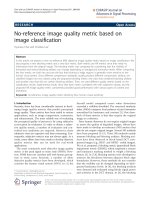
A new depth image quality metric using a pair of color and depth images

Multimed Tools Appl
DOI 10.1007/s11042-016-3392-4

A new depth image quality metric using a pair of color
and depth images
Thanh-Ha Le1 · Seung-Won Jung2 · Chee Sun Won3

Received: 17 July 2015 / Revised: 17 February 2016 / Accepted: 23 February 2016
© Springer Science+Business Media New York 2016

Abstract Typical depth quality metrics require the ground truth depth image or stereoscopic color image pair, which are not always available in many practical applications. In
this paper, we propose a new depth image quality metric which demands only a single pair
of color and depth images. Our observations reveal that the depth distortion is strongly
related to the local image characteristics, which in turn leads us to formulate a new distortion assessment method for the edge and non-edge pixels in the depth image. The local
depth distortion is adaptively weighted using the Gabor filtered color image and added up
to the global depth image quality metric. The experimental results show that the proposed
metric closely approximates the depth quality metrics that use the ground truth depth or
stereo color image pair.
Keywords Depth image · Image quality assessment · Reduced reference · Quality metric

Seung-Won Jung

Thanh-Ha Le

Chee Sun Won

1

University and Engineering and Technology, Vietnam National University, Hanoi, Vietnam

2

Department of Multimedia Engineering, Dongguk University, Pildong-ro 1gil, Jung-gu, Seoul
100-715, Korea

3

Department of Electronics and Electrical Engineering, Dongguk University, Pildong-ro 1gil,
Jung-gu, Seoul 100-715, Korea


Multimed Tools Appl

1 Introduction
Depth images play a fundamental role in many 3-D applications [6, 17, 24, 25]. For example,
depth images can be used to generate arbitrary novel viewpoint images by interpolating or
extrapolating the images at the available viewpoints. In addition, high quality depth images
open up opportunities to solve challenging problems in computer vision [13]. The depth
image can be obtained either by matching a rectified color image pair, i.e., stereoscopic
image, or by using depth cameras. In stereo matching techniques [19, 29], inaccurate depth
images are often produced because of occlusion, repeated patterns, and large homogeneous
regions. Although the inherent difficulty of stereo matching can be solved using the depth
camera [27], an inevitable sensor noise problem remains.
Owing to the widespread use of depth images, the quality assessment of depth images
becomes essential. One simple method of the depth image quality assessment is to compare
the depth image to be tested with its ground truth depth image [21]. This method corresponds to the full reference depth quality metric (FR-DQM), which can precisely measure
the accuracy of the depth image. However, the ground truth depth image is not always attainable in most practical applications. An alternative method is to evaluate the quality of the
reconstructed color image obtained using the depth image. For example, the right-viewpoint
image can be rendered by using the left-view image and depth image, and the rendered
image can be compared with the original right-viewpoint image [12]. However, such a color
image pair is not always obtainable in the depth-image-based rendering (DIBR) applications

[1, 5].
In this paper we introduce a new depth quality metric, which requires only a pair of color
and depth images and, thus, is a reduced reference DQM (RR-DQM). Here, we consider
the color image as the reduced reference for the depth quality assessment. To formulate
the depth quality metric we investigate the effects of various sources of depth distortions
and come up with a local measurement using the Gabor filter [2] and the smallest univalue
segment assimilating nucleus (SUSAN) detector [23]. The experimental results demonstrate that the proposed RR-DQM closely approximates the conventional DQMs that use
the ground truth depth information or stereo image pair.
This paper is an extended version of our conference paper [20]. Compared to [20], more
detailed description of the proposed metric is provided with extensive experimental verification. Moreover, the proposed metric is applied to the depth image post-processing technique
to show its usefulness.
The rest of the paper is organized as follows. The proposed RR-DQM is described in
Section 2. The experimental results and conclusions are given in Section 3 and Section 4,
respectively.

2 Proposed depth quality metric
A new depth image quality metric is designed for the case when the depth image is not used
in a stand-alone fashion but in a combined fashion with the color image. The combination
of color and depth images is often required in multi-view and 3-D video applications, where
the depth image is frequently used to render or synthesize color images at novel viewpoints.
In such applications, since the same local distortion of the depth image does not equally
affect the resultant color images, we need to consider the local distortion of the depth
image jointly with the local characteristics of the color image. For example, a pair of simple


Multimed Tools Appl

Fig. 1 (a)-(b) Synthetic image pair and (c) ground truth depth image

synthetic grayscale images of the size 400×400 is shown in Fig. 1a and b. Here, the square

region of Fig. 1a including horizontal, vertical, and two diagonal edges is left-shifted by
50 pixels as shown in Fig. 1b. In other words, the pixels inside the square have the same
horizontal disparity value as shown in Fig. 1c. The black background is located in the infinite distance, i.e. disparity value is zero. Note that the other directional disparities can be
ignored when the two images are rectified [14]. To analyze the effect of depth distortion, we
change the disparity values inside the square as shown in Fig. 2a and b. Precisely, one noisy
row is generated using the zero-mean uniform random distribution with a variance of 10.
The length of the row is the same as the width of the square, and the generated noisy row
is added to all the rows in the square of the depth image, resulting Fig. 2a. This can simulate depth distortion along the horizontal direction. Note that the depth values should be the
same along the vertical direction. The depth image with distortion along vertical direction
can be produced in a similar manner as shown in Fig. 2b.
Given a pair of color and depth images, the stereoscopic image can be obtained. Specifically, the pixels in the one viewpoint image can be found from the pixels in the other
viewpoint image in which the pixel positions are determined according to the disparity values in the depth image. From the synthesized color image, we can analyze the influence of
depth distortions. From Fig. 2c and d, one can notice that the horizontal image edges are
not seriously deteriorated. Since only the horizontal disparity is assumed, different directional distortions can change only the start and end positions of the horizontal edges. In
other words, the local distortion of the depth image in the horizontal edge regions does not
have a significant impact on the quality of the rendered image. It can be also found that the
distortion in the rendered images is prominent when the depth value varies along the image
edges. For example, the vertical image edges are severely damaged when the depth image
has distortion along vertical direction as shown in Fig. 2b and d.
From the above observations, it is found that the effect of local depth distortion is strongly
dependent on the local image characteristics. Thus, the relation between the depth distortion
and image characteristics should be exploited to measure the quality of the depth image.
Figure 3 shows the flowchart of the proposed RR-DQM in which the Gabor filter [2] is
used to weight differently according to the local image structures. In addition, the SUSAN
edge detector [23] is employed to attain the edge information of the image. In particular,
the SUSAN detector is known to robustly estimate image edges and their edge direction. Of
course, other edge detectors [15, 18] can be employed.


Multimed Tools Appl

Fig. 2 Distorted depth images and rendered grayscale images: (a) depth image with distortion along horizontal direction, (b) depth image with distortion along vertical direction, (c) rendered left-view image obtained
using Fig. 1b and a, g rendered left-view image obtained using Fig. 1b and b

The Gabor filter is a close model of the receptive fields [7, 28] and widely applied to
image processing applications. Let g denote the kernel of the Gabor filter defined as follows:
g(x, y) = exp −
where

xr2 + γ 2 yr2
2σ 2

cos 2π

xr
+φ ,
λ

(1)

xr = x cos θ + y sin θ
.
(2)
yr = −x sin θ + y cos θ
In (1) and (2), γ , σ , λ, φ and θ represent the aspect ratio, standard deviation, preferred
wavelength, phase offset, and orientation of the normal to the parallel stripes, respectively
[4]. Since the Gabor filter can be simply viewed as a sinusoidal plane wave multiplied by the


Multimed Tools Appl

Fig. 3 Flowchart of the proposed depth image quality metric

Gaussian envelope, especially for the edge and bar detection, antisymmetric and symmetric
versions of the Gabor filter [10] can be defined as
xr2 + γ 2 yr2
2σ 2

sin 2π

xr
,
λ

(3)

xr2 + γ 2 yr2
2σ 2

cos 2π

xr
.
λ

(4)

gedge (x, y) = exp −

gbar (x, y) = exp −

The edges and bars of the image, Iedge and Ibar , are obtained by convolving the original
image I with gedge and gbar , respectively. Here, the mean value of gbar is subtracted to
compensate for the DC component.
The filtered outputs are combined into a single quantity Iθ , called the Gabor engergy, as
follows:
Iθ (x, y) =

2 (x, y) + I 2 (x, y).
Ibar
edge

(5)

This Gabor energy approximates a specific type of orientation selective neuron in the primary visual cortex [9]. Figure 4 shows the Gabor energy results on Fig. 1a with various θ
values. In this example, γ and σ are set to 0.5 and 1.69 according to the default settings [4].
In addition, λ is adjusted to 3 and the Gabor energy outputs are scaled for the visualization.
As can be seen, the four directional components are successfully decomposed and the perceptually sensitive regions are distinguished. Thus, the Gabor energy of the image can be
exploited to adaptively weight the local distortion of the depth image.
In Fig. 2, we found that the influence of local depth distortion is strongly related to
edge direction. To this end, the SUSAN detector is used to extract edges and their directions. Detailed description and analysis of the SUSAN operator can be found in [23]. Let
EbI and EdI denote the edge map and edge direction map of the image I obtained using the
SUSAN detector, respectively. For simplicity, EdI is quantized to represent only the horizontal, vertical, left diagonal, and right diagonal directions. At the non-edge pixels, local depth
distortion is measured by the average difference of the depth values in the local neighborhood. On the other hand, at the edge pixels, depth variation along edge direction is measured
to consider edge distortion or deformation.


Multimed Tools Appl

Fig. 4 Gabor filtered results on Fig. 1a: (a) I0◦ , (b) I90◦ , (c) I135◦ , (d) I45◦

Let denote the depth distortion map obtained using the binary edge map EbI and the
depth image D:
⎧1
|D(x, y)−D(x +u, y +v)| ; if EbI (x, y) = 0
⎨8
(u,v)∈N
8
(x, y) =
,
(6)
⎩ D(x, y)− 1 (D(x +x , y +y )+D(x +x , y +y )) ; otherwise
1
1
2
2
2
where N8 represents the 8-neighborhood. At the non-edge pixels, the mean absolute difference (MAD) is used to measure local depth distortion. Meanwhile, at the edge pixels,
the average of the two adjacent depth values along the edge direction is differentiated with
the center pixel’s depth value. In other words, (xi , yi ) is determined according to the edge
direction. For example, (x1 , y1 ) = (1, 0) and (x2 , y2 ) = (−1, 0) for the horizontal edge. Note
that the central difference can distinguish an abrupt change from a gradual change. Thus, a


Multimed Tools Appl

natural change of depth values along edge direction caused by slanted surfaces is excluded
in the computation of local depth distortion.
When the depth image is captured by the depth camera, saturated pixels often appear in
highly reflective regions. Such saturated depth pixels have invalid depth values, and thus we

consider those pixels as outliers. Many stereo matching algorithms [21, 26] also identify the
outlier pixels without estimating their depth values. In the proposed method, if the neighboring pixel in (6) belongs to the outlier pixels, the corresponding position is excluded from
N8 . In a similar manner, for the edge positions, only one neighboring depth value is used if
one of two neighbors is outlier. Distortion estimation is not performed if both are outliers.
As the depth discontinuities along color image edges are the major source of local depth
distortion, both the local image characteristics (Iθ ) and local depth distortion ( ) are used
to obtain the global distortion map . To this end, is defined by merging Iθ and as
follows:
(x, y) =

αθ · Iθ (x, y) ·

(x, y),

(7)

θ∈

where = {0◦ , 45◦ , 90◦ , 135◦ } and αθ is the weight of the direction θ . Figure 5 shows the
resultant distortion maps obtained using Fig. 2a and b, where αθ = {1, 0.5, 0, 0.5} for the
four directions in . By comparing Figs. 2 and 5, it can be seen that the distortion maps are
highly correlated with visual geometric degradation caused by depth distortion.
Finally, the RR-DQM is defined by pooling all the distortion values in except for the
outlier regions,
⎛
⎞
1 ⎝
(8)
(x, y) ⎠,
DQMRR =

n(ϒ1 )
(x,y)∈ϒ1

where ϒ1 is a set of all pixels excluding the outlier pixels and n(ϒ1 ) is the cardinality of
ϒ1 . Note that the proposed RR-DQM requires only one pair of color and depth images.

Fig. 5 Global distortion maps corresponding to (a) Figs. 2a and (b) 2b


Multimed Tools Appl

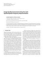
Fig. 6 Example on the Cones image: (a) original left-view image, (b) ground truth depth image, (c) ground
truth occlusion map, (d) LPCD distorted depth image with max =2, (e) compensated left-view image, (f)
error image excluding occluded region


Multimed Tools Appl

Fig. 7 Scatter plot of the RR-DQM versus depth distortion for random noise: (a) Cones, (b) T eddy, (c)
T sukuba, (d) V enus

3 Experimental results
The proposed RR-DQM mainly consists of the Gabor filer and the SUSAN detector with
some parameters. In the Gabor filter, γ and σ were set to 0.5 and 1.69, respectively (these are
the default values in typical applications of Gabor filters [4]). In addition, λ was empirically
determined as 3 by using test color-depth image pairs available in the Middlebury database
[21]. The brightness threshold and the kernel radius in the SUSAN operator were chosen to
15 and 3, respectively, according to [23].
In order to validate the proposed RR-DQM, the RR-DQM was compared with the conventional metrics. To this end, we used the Middlebury dataset, where the ground truth depth
image and stereo image pair are available. The two different types of the depth distortion

were simulated. First, the uniformly distributed random noise was added to the ground truth
depth image since the noisy depth images can approximate the depth images obtained by


Multimed Tools Appl

Fig. 8 Scatter plot of the RR-DQM versus prediction error for random noise: (a) Cones, (b) T eddy, (c)
T sukuba, (d) V enus

the depth camera. Second, the geometric distortion, local permutation with cancelation and
duplication (LPCD) [3], was applied to the depth image D by
D(x, y) = Dgt (x +

h (x, y), y

+

(9)

w (x, y)),

where Dgt denotes the ground truth depth image, h and w are the i.i.d. integer random variables uniformly distributed in the interval [− max , max ], and max controls the
amount of distortion. This local geometric distortion can simulate the inaccurate depth values in the object boundaries, where the stereo matching techniques usually find difficulty in
estimating depth values.
Given the degraded and ground truth depth images, the FR-DQM measures the difference
between two depth images as follows:
D(x, y) − Dgt (x, y)
DQMF R =

(x,y)∈ϒ2

n(ϒ2 )

2

,

(10)


Multimed Tools Appl

Fig. 9 Scatter plot of the RR-DQM versus depth distortion for the LPCD distortion: (a) Cones, (b) T eddy,
(c) T sukuba, (d) V enus

where ϒ2 denotes a set of the ground truth depth pixels. Alternatively, the depth accuracy
can be measured by warping one image using the depth image and comparing the warped
image with the original image. In our work, the right-view image of the stereo pair is warped
and the prediction error, DQMP red , is measured by
I l (x, y) − I r (x + D(x, y), y)
DQMP red =

(x,y)∈ϒ3

n(ϒ3 )

2

,

(11)

where I l and I r denote the left-view and right-view images, respectively. Here, ϒ3 indicates
a set of pixels in the left-view image except for the occluded pixels.
Figure 6 illustrates the above two metrics for the Cones image. In this example, the
LPCD distortion with max of 2 was applied to the ground truth depth image in Fig. 6b.
Then, the right-view image and the distorted depth image in Fig. 6d were used to reconstruct
the left-view image shown in Fig. 6e. DQMF R is the amount of the difference between
Figs. 6b and d in the non-outlier region, a white region in Fig. 6c. Similarly, the prediction error of the left-view image within the non-outlier region, shown in Fig. 6f, is used to


Multimed Tools Appl

Fig. 10 Scatter plot of the RR-DQM versus prediction error for the LPCD distortion: (a) Cones, (b) T eddy,
(c) T sukuba, (d) V enus

compute DQMP red . These two metrics, DQMF R and DQMP red , can accurately assess
the quality of the depth image by using the ground truth depth image and the stereo image
pair, respectively. Thus, our objective is to show strong correlation between the proposed
RR-DQM and these metrics.
Figure 7 shows the scatter plot of DQMRR versus DQMF R for the noisy depth images
using four stereo test images, Cones, T eddy, T sukuba, and V enus. In this test, 100 noisy
depth images were obtained by increasing the variance of the added noise from 1 to 100.
As can be seen, DQMRR has almost perfect linear relationship with DQMF R . Thus, the
proposed metric can accurately assess the amount of the noise in the depth image. The
relation between DQMRR and DQMP red for the same test images is shown in Fig. 8.
Since the prediction error depends on the characteristics of the image, the correlation is not
as strong as that in Fig. 7. However, there still exists strong linear relationship, where the
Pearson’s correlation coefficient, R 2 , approaches to 1. The relationships of DQMRR with
DQMF R and DQMP red for the LPCD distortion are shown in Figs. 9 and 10, respectively.

Here, 25 distorted depth images were generated by increasing max from 1 to 25. As can
be seen, the proposed technique provides the similar quality metric without requiring the
additional information of the ground truth depth or the stereo image pair.


Multimed Tools Appl

Fig. 11 The sensitivity of the proposed metric with various λ values. The R 2 scores are measured between
(a) DQMRR and DQMF R for random noise, (b) DQMRR and DQMP red for random noise, (c) DQMRR
and DQMF R for LPCD distortion, and (d) DQMRR and DQMP red for LPCD distortion, respectively

As aforementioned, we used the default parameter settings from [4, 23], and thus λ
in (1) and αθ in (7) are only empirically chosen parameters. Figure 11 shows the sensitivity of the RR-DQM with respect to λ values. Here we set αθ as {1, 0.5, 0, 0.5} and
extracted R 2 scores by the same manner as Figs. 7-10. The resultant R 2 score curves
were generally smooth and had a peak around 3. Similarly, Fig. 12 shows the sensitivity
of the RR-DQM with respect to α0o values. Here we set α45o =0.5, α90o =0, α135o =0, and
λ=3.0 and extracted the R 2 scores. We observed that the R 2 scores tend to converge when
α0o is around 1. Similar results were obtained when α45o =0.5, α90o =0.0, and α135o =0.5,
respectively.
We then applied the RR-DQM to more general outdoor images in the KITTI database [8]
in which the disparity images estimated using Displets method [11] are used as the depth
ground truth. Figure 13a depicts the color image 2 10 and Fig. 13b depicts its estimated
depth. Table 1 demonstrates that the proposed depth quality metric is strongly correlated
with the conventional metrics requiring the ground truth depth image for both depth distortion and prediction error. Thus, the proposed metric can be used to assess the depth image
quality when such information is not attainable.


Multimed Tools Appl

Fig. 12 The sensitivity of the proposed metric with various α0o values. The R 2 scores are measured between

(a) DQMRR and DQMF R for random noise, (b) DQMRR and DQMP red for random noise, (c) DQMRR
and DQMF R for LPCD distortion, and (d) DQMRR and DQMP red for LPCD distortion, respectively

Moreover, the proposed RR-DQM can be worked with the depth refinement algorithm.
In [31], an iterative depth refinement algorithm was proposed by using bilateral filtering.
In each iteration, the cost volume representing the depth probability is modified by bilateral filtering and the depth image is updated. Since no specific depth quality metric is
employed, the update process can be terminated when the number of iteration reaches the
predefined number or the change of the depth image is negligible. If the RR-DQM is used
as a termination criterion, the update process can be finished when the amount of the quality
improvement is saturated. Figure 14 shows the RR-DQM results for each iteration using the
Cones and T eddy images. In this test, in order to simulate the low resolution depth image,
the original depth image was down-sampled by a factor of 4 and then up-scaled to the original resolution with the nearest neighborhood interpolation. Then, the LPCD distortion with
max of 2 was applied to induce the depth distortion. As can be seen, the RR-DQM converges in a few iterations and thus the change of the RR-DQM is effectively used as the
termination criterion of the depth refinement algorithm.


Multimed Tools Appl

Fig. 13 A test image pair from KITTI database: (a) Color image and (b) its estimated disparity using [11]

Lastly, we applied the proposed RR-DQM to evaluate the performance of depth sensors.
To this end, we used the Kinect dataset [16, 22, 30, 32], which includes aligned pairs of
color and depth images captured by different depth sensors. In particular, 1449 and 3485 test
image pairs captured by the Kinect v1 and v2 sensors were used for RR-DQM measurement,
respectively. Figure 15 shows the first three test image pairs in the dataset. Because all the

Table 1 The R 2 scores for 10 image pairs in the KITTI database
Image ID

Random noise

LDPC distortion

depth distortion

prediction error

depth distortion

prediction error

0 10

0.999

0.992

0.978

0.990

2 10

0.999

0.996

0.983

0.985

4 10

0.999

0.993

0.983

0.996

5 10

0.999

0.992

0.975

0.997

7 10

0.998

0.989

0.983

0.964

8 10

0.999

0.988

0.977

0.993

9 10

0.998

0.978

0.978

0.972

15 10

0.999

0.992

0.981

0.992

17 10

0.999

0.991

0.980

0.988

19 10

0.997

0.991

0.985

0.981


Multimed Tools Appl

Fig. 14 The RR-DQM results of the depth refinement algorithm: (a) Cones and (b) T eddy

images were captured in indoor environments and the type and size of captured objects
are very similar, we can estimate the performance of the depth sensor by comparing the
average RR-DQM scores. The average RR-DQM scores of the Kinect v1 and v2 sensors
were obtained as 14.676 and 13.016, respectively, which illustrate the superiority of the

Kinect v2 sensor over the Kinect v1.

Fig. 15 The first three image pairs of the Kinect dataset [16, 22, 30, 32]. (a) Color (left) and depth (right)
image pairs captured by the Kinect v1 sensor, (b) color (left) and depth (right) image pairs captured by the
Kinect v2 sensor


Multimed Tools Appl

4 Conclusion
In this paper, we proposed a depth quality assessment technique that does not require the
ground truth depth image or the stereo image pair. Based on the analysis using the synthetic
image, the strong correlation between local depth distortion and the local image characteristic is verified. Then, the depth distortion is measured depending on the edge directions.
In addition, the Gabor filter is used to adaptively weight local depth distortion. The experimental results show that the proposed metric closely approximates the conventional depth
quality metrics that necessitate the additional information.
Since the color image is usually captured together with the depth image in the depth
camera applications, the proposed quality metric can be used to assess the performance of
the depth camera. Also, depth image refinement algorithms can adopt the proposed metric
for the termination criterion of the refinement. In depth based image rendering, the proposed
metric can be employed to predict the quality of the image to be rendered.
Acknowledgments Dr. Thanh-Ha Le’s work was supported by the basic research projects in natural science in 2012 of the National Foundation for Science & Technology Development (Nafosted), Vietnam
(102.01-2012.36, Coding and communication of multiview video plus depth for 3D Television Systems). Prof. Seung-Won Jung’s research was supported by Basic Science Research Program through the
National Research Foundation of Korea(NRF) funded by the Ministry of Science, ICT & Future Planning
(NRF-2014R1A1A2057970).

References
1. Chai B-B, Sethuraman S, Sawhney HS, Hatrack P (2004) Depth map compression for real-time viewbased rendering. Pattern Recogn Lett 25(7):755–766
2. Daugman J (1985) Uncertainty relation for resolution in space, spatial frequency, and orientation
optimized by two-dimensional visual cortical filters. Opt Soc Amer J A: Opt Image Sci 2:1160–1169
3. D’Angelo A, Barni M, Menegaz G (2007) Perceptual quality evaluation of geometric distortions in

images. In: Proceedings SPIE, Human Vision and Electronic Imaging XII, pp 1–12
4. D’Angelo A, Zhaoping L, Barni M (2010) A full-reference quality metric for geometrically distorted
images. IEEE Trans Image Process 19(4):867–881
5. Fehn C (2004) Depth-image-based rendering (DIBR), compression, and transmission for a new approach
on 3d-TV. In: Proceedings of SPIE, pp 93–104
6. Fehn C, De la Barr´e R, Pastoor S (2006) Interactive 3-DTV-concepts and key technologies. Proc IEEE
94(3):524–538
7. Gallant J, Braun J, Essen DV (1993) Selectivity for polar, hyperbolic, and cartesian gratings in macaque
visual cortex. Science 259(5091):100–103
8. Geiger A, Lenz P, Urtasun R (2012) Are We ready for Autonomous Driving? The KITTI Vision
Benchmark Suite. In: Conference on Computer Vision and Pattern Recognition
9. Grigorescu C, Petkov N, Kruizinga P (2002) Comparison of texture features based on Gabor filters.
IEEE Trans Image Process 11(10):1160–1167
10. Grigorescu C, Petkov N, Westenberg MA (2003) Contour detection based on nonclassical receptive field
inhibition. IEEE Trans Image Process 12(7):729–739
11. Guney F, Geiger A (2015) Displets: Resolving Stereo Ambiguities using Object Knowledge. In:
Conference on Computer Vision and Pattern Recognition
12. Ha K, Bae S.-H., Kim M (2013) An objective no-reference perceptual quality assessment metric based
on temporal complexity and disparity for stereoscopic video. IEIE Trans Smart Signal Comput 2(5):255–
265
13. Han J, Shao L, Xu D, Shotton J (2013) Enhanced computer vision with microsoft kinect sensor: a review.
IEEE Trans Cybern 43(5):1318–1334
14. Hartley RI (1999) Theory and practice of projective rectification. Int J Comput Vis 35(2):115–127


Multimed Tools Appl
15. Jain M, Gupta M, Jain NK (2014) The design of the IIR differintegrator and its application in edge
detection. J Inf Process Syst 10(2):223–239
16. Janoch A, Karayev S, Jia Y, Barron JT, Fritz M, Saenko K, Darrell T (2011) Acategory-level 3-d object
dataset: putting the kinect to work. In: Proceedings of ICCV Workshop on Consumer Depth Cameras for

Computer Vision, pp 1168–1174
17. Jung S-W (2014) Image contrast enhancement using color and depth histograms. IEEE Signal Process
Lett 21(4):382–385
18. Khongkraphan K (2014) An efficient color edge detection using the Mahalanobis distance. J Inf Process
Syst 10(4):589–601
19. Klaus A, Sormann M, Karner K (2006) Segment-based stereo matching using brief propagation and
a self-adapting dissimilarity measure. In: Proceedings of IEEE Conference on Pattern Recongnition,
pp 15–18
20. Le T-H, Lee S, Jung S-W, Won CS (2015) Reduced reference quality metric for depth images. In:
Proceedings Advanced Multimedia and Ubiquitous Engineering, pp 117–122
21. Scharstein D, Szeliski R (2002) A taxonomy and evaluation of dense two-frame stereo correspondence
algorithms. Int J Comput Vis 47(1-3):7–42
22. Silberman N, Hoiem D, Kohli P, Fergus R (2012) Indoor segmentation and support inference from rgbd
images. In: Proceedings of European Conference on Computer Vision, pp 746–760
23. Smith SM, Brady JM (1997) SUSAN-A new approach to low level image processing. Int J Comput Vis
23(1):45–78
24. Smolic A, Mueller K, Stefanoski N, Ostermann J, Gotchev A, Akar GB, Triantafyllidis G, Koz A (2007)
Coding algorithms for 3DTV-a survey. IEEE Trans Circ Syst Video Technol 17(11):1606–1621
25. Smolic A, Mueller K, Merkle P, Kauff P, Wiegand T (2009) An overview of available and emerging 3D
video formats and depth enhanced stero as efficient generic solution. In: Proceedings of 27th Conference
on Picture Coding Symposium, pp 389–392
26. Strecha C, Fransens R, Gool L. V (2006) Combined depth and outlier estimation in multi-view stereo.
In: Proceedings of IEEE Conference on Computer Vision and Pattern Recognition, pp 2394–2401
27. Um G.-M., Kim KY, Ahn C, Lee K. H (2005) Three-dimensional scene reconstruction using multiview
images and depth camera, pp 271–280
28. Vipparthi S, Nagar S (2014) Color directional local quinary patterns for content based indexing and
retrieval. Human-centric Comput Inf Sci 4(6):1–13
29. Wang Z-F, Zheng Z-G (2008) A region based stereoo matching algorithm using cooperative optimization. In: Proceedings of IEEE Conference on Computer Vision and Pattern Recongnition, pp 1–8
30. Xiao J, Owens A, Torralba A (2013) SUN3d: A database of big spaces reconstructed using SfM and
object labels. In: Proceedings International Conference on Computer Vision, pp 1–8

31. Yang Q, Yang R, Davis J, Nister D (2007) Spatial-depth super resolution for range images. In:
Proceedings of IEEE Conference on Computer Vision and Pattern Recognition, pp 1–8
32. Zhou B, Lapedriza A, Xiao J, Torralba A, Oliva A (2014) Learning deep features for scene recognition
using places database. In: Proceedings of Advances in Neural Information Processing Systems, pp 1–9

Thanh-Ha Le received the B.S. and M.S. degrees in information technology from College of Technology,
Vietnam National University, in 2005. He received the Ph.D. degree from the Department of Electronics
Engineering at Korea University. He is now a researcher with the Faculty of Information Technology, University of Engineering and Technology, Vietnam National University, Hanoi, Vietnam. His research interests
are video processing, image processing, robot vision, and robotics.


Multimed Tools Appl

Seung-Won Jung received the B.S. and Ph.D. degrees in electrical engineering from Korea University, Seoul,
Korea, in 2005 and 2011, respectively. He was a Research Professor with the Research Institute of Information and Communication Technology, Korea University, from 2011 to 2012. He was a Research Scientist
with the Samsung Advanced Institute of Technology, Yongin-si, Korea, from 2012 to 2014. He is currently
an Assistant Professor at the Department of Multimedia Engineering, Dongguk University, Seoul, Korea. He
has published over 40 peer-reviewed articles in international journals. His current research interests include
image enhancement, image restoration, video compression, and computer vision.

Chee-Sun Won received the B.S. degree in electronics engineering from Korea University, Seoul, in 1982,
and the M.S. and Ph.D. degrees in electrical and computer engineering from the University of Massachusetts,
Amherst, in 1986 and 1990, respectively. From 1989 to 1992, he was a Senior Engineer with GoldStar Co.,
Ltd. (LG Electronics), Seoul, Korea. In 1992, he joined Dongguk University, Seoul, Korea, where he is
currently a Professor in the Division of Electronics and Electrical Engineering. He was a Visiting Professor
at Stanford University, Stanford, CA, and at McMaster University, Hamilton, ON, Canada. His research
interests include MRF image modeling, image segmentation, robot vision, image resizing, stereoscopic 3D
video signal processing, and image watermarking.