DSpace at VNU: Effects of surface morphology and anisotropy on the tangential-momentum accommodation coefficient between Pt(100) and Ar

PHYSICAL REVIEW E 86, 051201 (2012)

Effects of surface morphology and anisotropy on the tangential-momentum accommodation
coefficient between Pt(100) and Ar
Thanh Tung Pham, Quy Dong To,* Guy Lauriat, and C´eline L´eonard
Universit´e Paris-Est, Laboratoire Modelisation et Simulation Multi Echelle, UMR 8208 CNRS, 5 Boulevard Descartes,
77454 Marne-la-Vall´ee Cedex 2, France

Vo Van Hoang
Department of Physics, Institute of Technology, National University of Ho Chi Minh City, 268 Ly Thuong Kiet Street,
District 10, Ho Chi Minh City, Vietnam
(Received 9 July 2012; published 26 November 2012)
In this paper, we study the influence of platinum (100) surface morphology on the tangential-momentum
accommodation coefficient with argon using a molecular dynamics method. The coefficient is computed directly
by beaming Ar atoms onto the surfaces and measuring the relative momentum changes. The wall is maintained
at a constant temperature and its interaction with the gas atoms is governed by the Kulginov potential. To capture
correctly the surface effect of the walls and the atoms’ trajectories, the quantum Sutton-Chen multibody potential
is employed between the Pt atoms. The effects of wall surface morphology, incident direction, and temperature
are considered in this work and provide full information on the gas-wall interaction.
DOI: 10.1103/PhysRevE.86.051201

PACS number(s): 47.45.Gx, 47.11.Mn

I. INTRODUCTION

In most applications concerning a fluid flowing past a
solid surface, no-slip conditions are usually employed: the
fluid velocity at the wall is assumed to be the same as the
surface velocity. This assumption, which works well in many
practical problems, breaks down when the channel height
under consideration is at a micro or nano length scale [1]. For

gases, Maxwell [2] introduced a gas-wall interaction parameter, the tangential-momentum accommodation coefficient σ , to
quantify the slip effects. He postulated that after collision with
the wall, a gas atom rebounds either diffusively or specularly,
with the associated portions of σ and (1 − σ ), respectively.
The slip velocity, vs , equal to the difference between the gas
velocity at the wall and the wall velocity, can be evaluated by
the following expression:
vs =

∂v
2−σ
λ
σ
∂z

,

(1)

w

| is the derivative of
where λ is the mean free path and ∂v
∂z w
the gas velocity at the wall surface. The latter is assumed to
be normal to the z direction. Although molecular dynamics
(MD) simulations showed that the reflection mechanism is
more complicated than Maxwell’s postulate, the coefficient σ
is still widely used due to its simplicity. In practice, a fully
accommodated coefficient, σ = 1, is frequently used whereas

experiments record smaller values ranging from 0.7 to 1.0 and
MD simulations results are even much smaller [3].
Based on Eq. (1), the σ parameter for a gas-wall couple
can be determined by either experiments [4] or molecular
dynamics [5,6] in the Navier-Stokes slip regime. However,
most MD simulations of flows were done at nanoscale [7]
and did not have the same conditions as in experiments.
In order to compare calculations with measurements for

*



1539-3755/2012/86(5)/051201(9)

dilute gases, a more relevant MD approach [8,9] consists of
studying every single gas-wall collision event. Consequently,
σ can be computed directly by projecting gas atoms onto the
surfaces and finding momentum changes [10]. This approach,
which is quite similar to beam experiments [11], provides
insights into the reflection mechanism and can be used to
improve Maxwell’s model. As far as multiscale simulations
are concerned, the obtained fluid-wall interaction results can
be coupled with other numerical methods [12–17].
We note that the term ( 2−σ
)λ in Eq. (1) is equivalent to
σ
the slip length under Navier slip boundary conditions and
the use of one parameter σ as in Maxwell’s model means
that the slip behavior is isotropic. For anisotropic textured

surfaces, more sophisticate models are needed to reproduce
the direction-dependent slip or gas-wall interaction behavior.
Bazant and Vinogradova [18] suggested using a slip length
tensor to quantify this behavior. The tensorial nature of
the slip effect was shown to be related to the interfacial
diffusion [18–21]. Effective slip tensors with bounds for
flows over superhydrophobic surfaces were also obtained
[22,23]. As the slip models describe macroscopic behaviors,
it is thus relevant to investigate the problem at the scale of
fluid-wall interaction. For gases, Dadzie and Meolans [24]
generalized Maxwell’s scattering kernel by using anisotropic
accommodation coefficients. The consequences of the model
on the slippage have not been studied. Since the anisotropic
scattering kernel model does not provide full information
about the gas-wall collisions, we use the MD method to
study these interactions in detail with the focus on the surface
morphology. The MD code used in this paper is the parallel
version described in Ref. [8]. The original code [25] has been
enriched (e.g., multibody potentials, statistical tools, etc.) to
adapt to the aim of the present work. The trajectory images
are obtained by using a molecular visualization program,
VMD [26].
Generally, results obtained from MD simulations depend
on the following factors.

051201-1

©2012 American Physical Society

´
PHAM, TO, LAURIAT, LEONARD,
AND HOANG

PHYSICAL REVIEW E 86, 051201 (2012)

(i) The interaction potential between the gas and wall
atoms.
(ii) The dimension of the simulation models. In general,
three-dimensional (3D) models are better than 2D models since
three dimensions account for interactions of the gas atom with
all its neighbors.
(iii) The potential between the solid atoms must be good
enough to reproduce the free surface effect. It is well known
that the distance between the atomic layers near the free surface
is much smaller than in the bulk.
(iv) The temperature effect must be considered because gas
molecules are adsorbed easier at cold walls than at hot walls,
which can result in a higher σ .
(v) The surfaces are not always ideally smooth and can
have different morphologies (e.g., randomly rough or textured
surfaces).
This work aims at including these features in simulations
of molecular beam experiments. The gas-wall couple under
consideration is argon and platinum but the methodology of the
present work can be used to obtain σ for any gas-wall couple
provided that an appropriate potential is used. The paper is
organized as follows. After the Introduction, Sec. II is devoted
to the description of the computational method. It discusses
briefly the choice of potentials, the method to prepare surface

samples, and the MD simulation of the gas-wall interaction.
We remark that a part of surface sample preparation requires a
separate MD simulation of film deposition processes in order
to create a realistic random roughness surface. The σ results
obtained from the calculations are then shown in Sec. III.
Finally, conclusions and perspectives are discussed in Sec. IV.

TABLE I. Parameters of the Pt-Ar pairwise potential [27].
V0 (eV)

˚ −1 )
α (A

˚
R0 (A)

˚ 6)
C6 (eV · A

20 000

3.3

−0.75

68.15

and the results (e.g., equilibrium distance, potential well depth,
etc.) are compared with several existing potentials for the Ar-Pt
couple.

In terms of the potential between the Pt atoms, the
multibody quantum Sutton-Chen (QSC) potential is used
[32]. As a particular Finnis-Sinclair potential type, the QSC
potential includes quantum corrections and predicts better
temperature-dependent properties. For a system of N Pt atoms,
the potential is given by the following expression:
N

i=1

a
Rij

ρi =
j =1
j =i

a
Rij

j =1
j =i

N

n

1/2

−c

ρi

,

i=1

(3)

m

,

where a is the lattice constant, Rij is the distance between
atom i and atom j , and ρi is the local density of atom i.
The parameters and a are the scales of energy and length,
respectively, and n and m are the range and shape of the
potential, respectively. These potential parameters are given
in Table II. Combining the Ar-Pt and Pt potentials, we can
compute the total potential of the system by
N

Epot =

A. Interatomic potential

φAr−Pt (RAr−i ) + Epot,Pt ,

(4)

i=1

The interatomic potentials play an important part in the MD
simulations since they govern the dynamics of the system and
thus the accuracy of the results. In this work, the following
van der Waals type pair potential between At and Pt derived
by Kulginov et al. [27] is used:

RAr−Pt = |rAr − rPt |,

N

N

II. COMPUTATION MODEL

φAr−Pt (RAr−Pt ) = V0 e−α(RAr−Pt −R0 ) −

1
2

Epot,Pt =

C6
,
6
RAr−Pt

(2)

where RAr−Pt is the distance between an Ar atom at location rAr
and a Pt atom at location rPt . Contrary to the usual LennardJones potentials, the repulsive part of this pair potential has
a Born-Mayer form and provides a better description of
the strong repulsion of the electrons. The pairwise potential
parameters have been empirically adjusted such that the
laterally average potential reproduces the measured properties
of an Ar atom adsorbed on a slab of Pt atoms, i.e., a well
depth of about 80 meV [28] and a vibrational frequency of
the adsorbed atom of about 5 meV [29]. The van der Waals
interaction of an Ar atom with a platinum surface can be
evaluated from the Ar polarizability and the Pt dielectric
function. The values of the potential parameters are given
in Table I and are in good agreement with an ab initio based
calculation [30]. In Ref. [30], the CRYSTAL09 software [31] was
used to study the interaction between Ar and Pt(111) surfaces,

and we can compute the force fi acting on atom i at position
ri by
fi = −

∂Epot
.
∂ri

(5)

Since we only consider the interaction of one Ar atom with
a Pt surface, there is no contribution of the Ar-Ar term in
the total potential formula Epot . The accuracy of the QSC
potential for Pt has been justified in Ref. [33] as it reproduces

accurately the melting temperature and the specific heat of
the material. Although its implementation is more costly than
the harmonic (spring) potential, it should better reproduce the
surface effects, since atoms near the free surfaces are different
from the bulk. Our tests on the QSC potential show that, in
a fully relaxed equilibrium system, the interatomic distance
near the free surfaces is much smaller than that in the bulk
(see Fig. 1). As shown by previous works [34–36], the lattice
constant, wall mass, and stiffness can have significant impact
on σ and the slip effects.
TABLE II. Quantum Sutton-Chen parameters for Pt [33].
n

m

11

7

051201-2

(eV)
9.7894 × 10−3

c

˚
a (A)

71.336

3.9163


EFFECTS OF SURFACE MORPHOLOGY AND ANISOTROPY . . .

PHYSICAL REVIEW E 86, 051201 (2012)

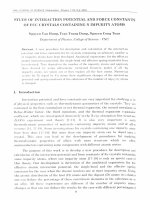
FIG. 1. (Color online) Surface effects: The fully relaxed configuration (right) is different from initial configuration (left). The solid
film system is composed of fixed atoms (bottom layer), thermostat
atoms (upper bottom layer), and normal atoms (remaining layers).
B. Surface samples

In this paper, three types of surfaces are considered: smooth
surfaces, periodic nanotextured surfaces, and randomly rough
surfaces. The orientation of their free surfaces is (100)
according to the Miller index. Initially, the Pt atoms are
arranged in layers and the two lowest ones (phantom atoms)
are used to fix the system and for the thermostat purpose. The
remaining Pt atoms are free to interact with other solid atoms
and gas atoms. The random arrangement of these atoms defines
the “rough” state of the surface and is detailed later on.
A smooth surface model is a system composed of 768 atoms
arranged in six layers, all of which are in perfect crystal order.
The nanotextured models are constructed from the smooth
surface model by successively adding atom layers to create
pyramids with a slope angle of 45◦ . The slope is necessary to
assure the stability of the system since perfectly vertical blocks
(slope angle 90◦ ) are less stable: in many cases atoms migrate
to lower positions and the blocks evolve into steplike structures

with smaller potential energy. The base of the pyramid can be
a square (type A, Fig. 2) or an infinite strip (type B, Fig. 3), so
that both isotropic and anisotropic effects can be considered.
Although these pyramids are simplified models of a real rough

FIG. 2. Nanotextured surface of type A (square).

FIG. 3. Nanotextured surface of type B (strip).

surface, they can show the dependence of σ on the roughness.
The latter in MEMS (microelectromechanical systems) or
NEMS (nanoelectromechanical systems) is reported to be
˚ [1]. In this work, the highest peak, varying with
several A
the number of atom layers added on the surfaces, ranges from
˚
2 to 6 A.
Randomly rough surface models are also constructed by
adding atoms to the smooth surfaces in a random way. In
the available literature, there are several mathematical models
[37–40] that describe random roughness. However, these
models are not suitable at the atomic scale: it is difficult to force
atoms to be at given positions and structure parameters such
as orientation (100) and lattice constant must be respected.
Furthermore such atomistic systems might not be appropriate
in terms of potential energy. In our opinion, a randomly rough
surface which is consistent with the internal atomistic structure
should be built from MD simulations. Rapid cooling of thin
films from the liquid state [41] can create rough surfaces but
the final systems could contain many defects (e.g., pores and

dislocations) and noncrystalline structure. As the paper focuses
on Pt(100), the rough surfaces are constructed by deposing
atoms randomly on the existing smooth platinum surface.
Since this procedure is quite similar to vapor-deposition
processes of films, it is assumed that the created surface is
quite close to real MEMS and NEMS surfaces. The procedure
of the material deposition is described as follows.
The initial system is a Pt plate made of four layers of 512
solid atoms, arranged in (100) fcc order. First, the system is
relaxed towards the minimum potential energy configuration.
Then, after 2000 time steps of 1 fs, a Pt atom is inserted

051201-3


´
PHAM, TO, LAURIAT, LEONARD,
AND HOANG

PHYSICAL REVIEW E 86, 051201 (2012)

FIG. 4. (Color online) Snapshot of deposition process (left) and
final thin film system (right).

˚ with the initial thermal
randomly from a height of 10 A
velocity corresponding to 1000 K. Under the attraction force
(QSC potential) from the Pt plate, the deposed Pt atoms move
downwards until they reach the plate which is maintained at
50 K (see a snapshot of the deposition process in Fig. 4).

Finally, when all inserted Pt atoms are attached firmly into the
Pt plate, the whole system undergoes the anneal process at the
ambient temperature Ta = 300 K with a time step equal to 2 fs.
During the whole simulation, the Verlet leap-frog integration
scheme is employed and the temperature is kept constant by a
simple velocity scaling method. Figure 4 shows a snapshot of
the final system whose total number of Pt atoms has reached
733. To improve the statistical results, five samples obtained
thanks to the above-described procedure are collected, as
shown in Fig. 5.
C. Dynamics of the gas-wall collision

In what follows, we describe the MD method used to
simulate the gas-wall collision and to calculate the σ coefficient. The simulations are three dimensional: an Ar atom is
projected onto a Pt(100) surface with different incident angles
θ and with different approaching ϕ planes. In the spherical
coordinate system, θ and ϕ are the polar and azimuthal
angles, respectively (see Fig. 6). The directional σdir coefficient
associated with each θ and ϕ is defined by the following

FIG. 5. (Color online) Five samples obtained from the deposition
process.

FIG. 6. Representation of θ and ϕ in the Cartesian coordinate
system.

formula [1]:
σdir (θ,ϕ) =

vin − vrn

,
vin

(6)

where vin and vrn are the projections of the incident velocity
and the reflected velocity on the vector n, respectively. The
latter is the intersection of the xOy plane and the ϕ plane;
i.e., it lies on xOy and makes an angle ϕ with respect to
Ox. Only one gas-wall collision is treated per simulation
and the averages vin and vrn in Eq. (6) are taken over a
large number of simulations (or collisions). The definition (6)
is the most accurate description of the gas-wall interaction
since it is associated with each direction. We also calculate
the effective anisotropic σan (ϕ) coefficients using the same
equation, Eq. (6), but with gas atoms arriving from all
directions: the direction of vi is randomly uniform with
vin > 0. In the special case where the surface is isotropic,
σan varies little with ϕ and a single effective isotropic σiso
constant is sufficient for modeling the gas-wall interaction as
in Maxwell’s model. The latter effective isotropic coefficient
is obtained by a similar method but vin and vrn in Eq. (6)
are further averaged over n (or ϕ).
We assume first that an Ar atom only interacts with the
˚ (see Fig. 7).
Pt wall within a cutoff distance of rc = 10 A
Since this distance is much smaller than the typical mean free
path at atmospheric pressure or in high vacuum (λ > 69 nm),
it can justify the choice of such a small region to calculate
˚ an Ar atom can

the σ coefficients. At a distance of 10 A,
be considered as noninteracting with the Pt wall atoms since
the potential value at that distance (−0.058 0736 meV) is
negligibly small when compared with the potential well depth
(10.21 meV). At the beginning of each simulation, an Ar
atom is inserted randomly at the height rc above the wall
surface with the initial incident velocity vi . The norm of
vi is equal to the thermal speed corresponding to the gas
beam temperature Tg . Although the results of this work are
obtained using a constant incident velocity corresponding
to the gas temperature, we have done separate simulations
using the Maxwell-Boltzmann velocity distribution and have
found that σ is insensitive to this modification. A collision is
considered as finished when the atom bounces back beyond

051201-4


EFFECTS OF SURFACE MORPHOLOGY AND ANISOTROPY . . .

PHYSICAL REVIEW E 86, 051201 (2012)
TABLE III. σdir (θ,ϕ) computed for the wall of type A at Tw = 200
K, 300 K, and 400 K for three roughness heights h with θ = 10◦ , 45◦ ,
and 80◦ and ϕ = 0◦ .
θ

Tw = 200 K

Tw = 300 K

Tw = 400 K

˚
A (h = 5.88 A)

10◦
45◦
80◦

0.96
0.92
0.90

0.87
0.85
0.83

0.79
0.77
0.74

˚
A (h = 3.92 A)

10◦
45◦
80◦

0.94
0.90

0.88

0.84
0.79
0.78

0.75
0.74
0.72

Smooth

10◦
45◦
80◦

0.85
0.82
0.80

0.72
0.70
0.69

0.61
0.60
0.59

Surface type

FIG. 7. Molecular dynamics scheme. The incident argon atoms
are with vi velocities. θ is the incident angle. The Pt wall has a fcc
structure with a (100) surface. The Pt atoms are controlled by the
Sutton-Chen potential.

the cutoff distance. Then the reflected velocity vr is recorded
for the statistical purpose and another Ar atom is reinserted
randomly to continue the process. After approximatively
10 000 collisions (simulations), converged values of σ values
were obtained. Numerical tests show that the statistical error
of a typical 10 000-collision average is within 1.0%.
Throughout the simulations, periodic boundary conditions
are applied along the x and y directions. The velocities and
positions of the gas atoms and the solid atoms at each time step
are calculated by the usual Verlet leap-frog integration scheme.
To control the temperature Tw of the system, the phantom
technique is used: the Langevin thermostat [42] is applied to
the atom layer above the fixed layer. The motion of an atom i
belonging to this layer is governed by the equation
mi

dvi (t)
= −ξ vi (t) + fi (t) + Ri (t).
dt

(7)

In Eq. (7), vi is the velocity of the atom i, fi is the resulting
force acting on it by the surrounding ones, mi is the atomic
mass, and ξ is the damping coefficient. The third term Ri in the

right-hand side of Eq. (7) is the random force applied on the
atom. In the simulation, it is sampled after every time step δt
from a Gaussian
√ distribution with a zero average and a mean
deviation of 6ξ kB Tw /δt. The simulations were carried out
by setting the time step and the damping factor at the following
values:
δt = 2fs,

ξ = 5.184 × 10−12 kg/s.

III. MD SIMULATION RESULTS
A. Effects of temperature and roughness height

From the description of the models in Sec. II, the coefficient
σdir can depend on the several input parameters: temperature,
surface morphology, and incident direction (θ,ϕ). The variation of σdir in terms of these parameters is investigated in the
following subsections.
The σdir results at different temperatures are shown in
Table III and Fig. 8. A general trend can be noticed here:
σdir increases as the temperature decreases, ranging from
0.78 to 0.92 in the case of the highest roughness considered
˚ This trend in σdir variation can be explained
(h = 5.88 A).
by the fact that the adsorption is stronger with colder walls.
Gas atoms stay longer near the wall and interact more with
solid atoms, and, as a result, the reflection is more diffusive.
Similar remarks have been reported in Refs. [6,43] for confined
˚ and Tw = 300 K, Table IV shows that
systems. For h = 5.88 A

the σdir value varies very little with the incident angle θ and
is very close to the average isotropic value σiso = 0.85. This
means that for this kind of surface, Maxwell’s one-parameter
model is sufficiently accurate to model gas-wall interaction.
The σdir coefficient increases with the roughness of the
wall surface (see Table III and Fig. 8). Computations carried

(8)

The wall temperature Tw was kept at 200 K, 300 K, and 400
K and the gas beam temperature Tg was kept at a slightly
higher value than Tw , here Tg = 1.1Tw . Such choice of Tg was
made arbitrarily and the procedure of the present work can be
applied to any gas temperature. Generally, to obtain the best
statistical results, a typical run requires 4 × 107 time steps
of 2 fs. All simulations were run on nine processors, using
a domain decomposition and the message passing interface.
The longest simulation takes about 20 CPU h. We carried out
computations with different time steps from 1 to 3 fs and we
found that the results are insensitive to this factor.

FIG. 8. (Color online) σdir computed for the wall of type A
(square) at Tw = 200 K, 250 K, 300 K, 350 K, and 400 K for three
roughness heights h with θ = 45◦ and ϕ = 0◦ .

051201-5


´
PHAM, TO, LAURIAT, LEONARD,

AND HOANG

PHYSICAL REVIEW E 86, 051201 (2012)

TABLE IV. σiso and σdir (θ,ϕ) computed at Tw = 300 K.
Surface type

ϕ

θ

σdir

σiso

˚
A (h = 5.88 A)

0◦
0◦
0◦
0◦
0◦
–

10◦
30◦
45◦
60◦
80◦

–

0.87
0.86
0.85
0.85
0.83
–

–
–
–
–
–
0.85

Random
(Fig. 5)

–

–

–

0.92

Smooth

–

–

–

0.70

FIG. 10. (Color online) Typical collision trajectories (solid and
dashed lines) on a rough surface. Gas molecules move within the
valley between the peaks.
B. Surface anisotropy effect

out for pyramidal structures at a temperature of 300 K show
that the σdir coefficient can reach up to 0.87 for surfaces with
the highest peak configuration. It is clear that the presence of
peaks leads to nonuniform surface potentials with local minima
where gas molecules can easily be trapped: the gas atoms stay
longer near the wall, interact more with it, and lose their initial
momentum. Moreover, the changes in local wall slopes produce more or less random variations in the local incident and
reflection angles. Visualization of collision trajectories shows a
clear difference between a smooth surface and a rough surface.
On a smooth surface, a gas molecule collides and bounces several times before finally escaping from the influence distance rc
of the wall (see Fig. 9). On a rough surface, it stays near the wall
and moves within the valley between the peaks, a mechanism
similar to surface diffusion, until the wall provides enough energy to escape (see Fig. 10). The real behaviors are mixed: we
sometimes observe the colliding and bouncing mechanisms on
rough surfaces (not shown in Fig. 10), but they are not typical.
Next we considered the case of random surfaces obtained
from the atom deposition process. With the same parameters as
for the deposition process, the σdir values obtained for the five

samples shown in Fig. 5 exhibit small differences, from 0.90
to 0.93. It is very close to the σiso value for random surfaces,
0.92 (see Table IV). Thus, in addition to the roughness height,
the in-plane random arrangement of the atoms also plays a
significant role in the accommodation coefficient.

FIG. 9. (Color online) Typical collision trajectories (solid and
dashed lines) on a smooth surface. Gas molecules collide and bounce
several times before escaping.

An anisotropic textured surface can obstruct or facilitate
the flows differently along different directions. Bazant and
Vinogradova [18] generalized Navier slip boundary conditions
for anisotropic textured surfaces by using a tensorial slip
length. In the framework of the kinetic theory, Dadzie and
Meolans [24] proposed a new scattering kernel that accounts
for surface anisotropy. Their formulation is based on three
independent accommodation coefficients αx , αy , and αz along
the three directions: x, y, and z. The coefficients αx and
αy represent the tangential accommodation coefficients and
αz is the normal accommodation coefficient. The tangential
accommodation coefficient αn in direction n is then computed
by the following expression (see the Appendix):
σan (ϕ) = αn = αx cos2 ϕ + αy sin2 ϕ.

(9)

We remark that by substituting ϕ = 0◦ and ϕ = 90◦ , the
accommodation values αx and αy along the x and y directions
can be recovered. In this subsection, we study the anisotropy

effect using MD and the directional σ definition in Eq. (6) and
we examine the relation (9). The anisotropy effect can be seen
from Figs. 11 and 12: the σdir variation with ϕ is nonuniform for

FIG. 11. (Color online) σdir computed for type B walls (strip)
versus the azimuthal angle ϕ for different roughnesses (Tw = 300 K,
θ = 45◦ ). The solid lines are the analytical expressions (9) used to fit
the present numerical results.

051201-6


EFFECTS OF SURFACE MORPHOLOGY AND ANISOTROPY . . .

PHYSICAL REVIEW E 86, 051201 (2012)
TABLE V. Ratio vrm / vrn computed for type B walls (strip)
with different roughness heights h at Tw = 300 K, θ = 45◦ , and
ϕ = 45◦ .
h

vrm / vrn

0
˚
1.96 A
˚
3.92 A
˚
5.88 A

0
0.15
0.39
0.67

IV. CONCLUDING REMARKS

FIG. 12. (Color online) σan computed for type B walls (strip)
versus the azimuthal angle for different roughnesses (Tw = 300 K).
The solid lines are the analytical expressions (9) used to fit the present
numerical results.

rough surfaces. The accommodation processes along the two
directions x and y are highly different. The σdir is minimum
when the atoms are projected along the longitudinal direction
of the strip (ϕ = 90◦ ), since the surface may be considered as
almost smooth in that direction (see Fig. 3). This σdir value
corresponds to αy in the model of Ref. [24]. The maximum
σdir values recorded for ϕ = 0◦ and h > 0 can be attributed to
the largest roughness effect in that direction and correspond
to αx in the model [24]. Moreover, Figs. 11 and 12 show
an increase of anisotropy effect as the roughness increases:
the difference between the highest σdir value and the smallest
σdir value increases with the roughness height whereas the σdir
results depend very little on the beaming direction for a smooth
surface. This could be explained by the fact that the smooth
surface can be considered isotropic. Although Figs. 11 and 12
show discrepancies of σdir values obtained in different ways,
all points can fit reasonably well the analytical relation (9).
For anisotropic surfaces, the reflected flux is not always

lying in the same plane with the arriving one. Consequently,
in addition to Eq. (6), we should account for the ratio of the
reflected flux components along the two orthogonal directions
m and n: vrm / vrn . According to the anisotropic model (see
Appendix), this ratio can be computed by the expression
vrm / vrn =

(αx − αy ) cos ϕ sin ϕ
.
1 − αx cos2 ϕ − αy sin2 ϕ

In this paper, we have studied the effects of temperature,
surface texture, and anisotropy on the σ coefficient. The
computation model is based on the molecular beam experiments and constructed with the accurate available potentials
and interaction models. Although σ is not simply a gas-wall
constant, the MD result range agrees quite well with the experimental range at the ambient temperature. The randomly rough
surface obtained from the atomic deposition simulation is also
investigated in the paper. Concerning the anisotropy effect,
results on systems with anisotropic surfaces show that σ varies
significantly with orientation. Effective σ coefficients are obtained and compared with the available model in the literature.
APPENDIX: ANISOTROPIC SCATTERING KERNEL

For the gas-wall interaction, Dadzie and Meolans [24]
proposed an anisotropic scattering kernel B(v ,v) defined by
B(v ,v) =

μk Bk (v ,v)

(A1)

k

in which
μij = αi αj (1 − αk ), μi = αi (1 − αj )(1 − αk ),
μij k = αi αj αk ,
μ0 = (1 − αi )(1 − αj )(1 − αk ), i,j,k = x,y,z,

(A2)

i = j = k = i.
The vectors v ,v are, respectively, the arriving velocity and
the reflected one and the constants αx , αy , and αz are the
accommodation coefficients along the directions x, y, and
z. The elementary kernels Bk are given by the following
expressions:
B0 (v ,v) = δ(vz + vz )δ(vx − vx )δ(vy − vy ),
Bxy (v ,v) =

(10)
Biz (v ,v) =

By observing the surface structure, we can deduce that
vrm / vrn must vanish for impinging fluxes parallel to the
planes of symmetry of the anisotropic surface. That remark
is in good agreement with Eq. (10), where vrm / vrn = 0 at
ϕ = 0◦ and 90◦ . Our MD simulation confirms the remark and
also shows that the ratio is nonzero at ϕ = 0. From Table V, at
ϕ = 45◦ , we find that the ratio is significant. It even increases
as the roughness height increases; i.e., the anisotropic effect is
enhanced.

051201-7

Bxyz (v ,v) =
Bi (v ,v) =
Bz (v ,v) =
i,j =

1
2
2
2
δ(vz + vz )e−(vy +vx )/Cw ,
2
π Cw
2
2
2
2
√ 3 vz δ(vj − vj )e−(vi +vz )/Cw ,
π Cw
2
2
2
2
2
vz e−(vx +vy +vz )/Cw ,
(A3)
4
π Cw
1

2
2
δ(vz + vz )δ(vj − vj )e−vi /Cw ,
√
π Cw
2
2
2
vz δ(vi − vi )δ(vj − vj )e−vz /Cw ,
2
Cw
x,y, i = j,


´
PHAM, TO, LAURIAT, LEONARD,
AND HOANG

PHYSICAL REVIEW E 86, 051201 (2012)

where δ is the Dirac δ and Cw is a velocity constant depending
on the wall temperature. The boundary conditions for the
particle distribution function f (v) are then defined by
vz f (v) =

|vz |f (v )B(v ,v)dv ,
(A4)

= R × R × R− .
−

j

Since αx and αy are accommodation coefficients, we can
deduce the relations

=

+
j

−

m|vz |vj f (v )dv ,

=

+

with f and f being the velocity distribution associated with
the incident molecules and the reflected molecules. Dadzie and
Meolans [24] proved the following relation:
−
−
j

+
j

= αj , j = x,y,z.

(A6)

Their model is based on three parameters, αx , αy , and αz ,
defined along given directions of a system of coordinates. We
are interested in the accommodation coefficients in an arbitrary
direction. Hence, we consider a family of orthogonal directions
(n and m) obtained by rotating xOy around Oz by the angle
ϕ. Consequently, the n and m components are related to the x
and y components by
±
n

= cos ϕ

±
x

+ sin ϕ

±
y,

±
m

+ βnm

−
m,

+
m

= (1 − αm )

−
m

+ βnm

−
n,

αn = αx cos2 ϕ + αy sin2 ϕ,

m|vz |vj f (v)dv,

= R×R×R ,

−
j

−
n

(A8)

βnm = (αx − αy ) cos ϕ sin ϕ,

+

+

−

= (1 − αn )

with

+
j

We use
and
to denote the incoming flux at the wall of
the momentum j component. Then
−
j

+
n

= − sin ϕ

±
x

+ cos ϕ

±

y.

(A7)

[1] G. Karniadakis, A. Beskok, and N. Aluru, Microflows and
Nanoflows: Fundamentals and Simulation (Springer, New York,
2005).
[2] J. C. Maxwell, Philos. Trans. R. Soc. London 170, 231 (1879).
[3] B. Y. Cao, J. Sun, M. Chen, and Z. Y. Guo, Int. J. Mol. Sci. 10,
4638 (2009).
[4] E. B. Arkilic, K. S. Breuer, and M. A. Schmidt, J. Fluid Mech.
437, 29 (2001).
[5] Q. D. To, C. Bercegeay, G. Lauriat, C. L´eonard, and G. Bonnet,
Microfluid. Nanofluid. 8, 417 (2010).
[6] B. Y. Cao, M. Chen, and Z. Y. Guo, Appl. Phys. Lett. 86, 091905
(2005).
[7] Q. D. To, T. T. Pham, G. Lauriat, and C. L´eonard, Adv. Mech.
Eng. 2012, 580763 (2012).
[8] D. Rapaport, The Art of Molecular Dynamics Simulation
(Cambridge University Press, Cambridge, UK, 2004).
[9] M. Allen and D. Tildesley, Computer Simulation of Liquids
(Oxford University Press, London, 1989).
[10] G. W. Finger, J. S. Kapat, and A. Bhattacharya, J. Fluids Eng.
129, 31 (2007).
[11] C. T. Rettner, IEEE Trans. Magn. 34, 2387 (1998).
[12] G. Bird, Molecular Gas Dynamics and the Direct Simulation of
Gas Flows (Clarendon, Oxford, 1994).
[13] W. Liou and Y. Fang, Microfluid Mechanics (McGraw-Hill, New
York, 2003).

(A9)

αm = αy cos ϕ + αx sin ϕ,
2

2

and compute the accommodation coefficient along any direction n. For example, by setting the component −
m =0
(e.g., we beam atoms along direction n only), we can recover
the expression for αn in Eq. (9). The ratio between the
reflected components m and n can also be computed by the
expression
+
m/

+
n

=

(αx − αy ) cos ϕ sin ϕ
βnm
=
. (A10)
1 − αn
1 − αx cos2 ϕ − αy sin2 ϕ

It is clear that for the isotropic model αx = αy , this ratio
is always zero for all ϕ. Thus for the anisotropic surface

+
αx = αy , the ratio +
m / n is a function of ϕ and only
◦
vanishes at ϕ = 0 and 90◦ . For example, at ϕ = 45◦ , we
obtain
αx − αy
+
+
.
(A11)
m/ n =
2 − αx − αy

[14] H. Struchtrup, Macroscopic Transport Equations for Rarefied Gas Flows: Approximation Methods in Kinetic Theory
(Springer, New York, 2005).
[15] M. Kalweit and D. Drikakis, J. Comput. Theor. Nanosci. 5, 1923
(2008).
[16] M. Kalweit and D. Drikakis, Proc. Inst. Mech. Eng., Part C 222,
797 (2008).
[17] M. Kalweit and D. Drikakis, Mol. Simul. 36, 657 (2010).
[18] M. Z. Bazant and O. I. Vinogradova, J. Fluid Mech. 613, 125
(2008).
[19] N. V. Priezjev, J. Chem. Phys. 135, 204704 (2011).
[20] L. Bocquet and J. L. Barrat, Phys. Rev. E 49, 3079 (1994).
[21] L. Bocquet and J. L. Barrat, Soft Matter 3, 685 (2007).
[22] F. Feuillebois, M. Z. Bazant, and O. I. Vinogradova, Phys. Rev.
Lett. 102, 026001 (2009).
[23] F. Feuillebois, M. Z. Bazant, and O. I. Vinogradova, Phys. Rev.
E 82, 055301 (2010).

[24] S. K. Dadzie and J. G. Meolans, J. Math. Phys. 45, 1804
(2004).
[25] The source code is available for download at
/>[26] W. Humphrey, A. Dalke, and K. Schulten, J. Mol. Graphics 14,
33 (1996).
[27] D. Kulginov, M. Persson, C. T. Rettner, and D. S. Bethune, J.
Chem. Phys. 100, 7919 (1996).

051201-8


EFFECTS OF SURFACE MORPHOLOGY AND ANISOTROPY . . .
[28] M. Head-Gordon, J. C. Tully, C. T. Rettner, C. B. Mullins, and
D. Auerbach, J. Chem. Phys. 94, 1516 (1991).
[29] P. Zeppenfeld, U. Becher, K. Kern, R. David, and G. Comsa,
Phys. Rev. B 41, 8549 (1990).
[30] C. L´eonard, V. Brites, T. T. Pham, Q. D. To, and G. Lauriat
(unpublished).
[31] R. Dovesi, R. Orlando, B. Civalleri, C. Roetti, V. Saunders, and
C. Zicovich-Wilson, Z. Kristallogr. 220, 571 (2005).
[32] A. P. Sutton and J. Chen, Philos. Mag. Lett. 61, 139 (1990).
[33] S. K. R. S. Sankaranarayanan, V. R. Bhethanabotla, and B.
Joseph, Phys. Rev. B 74, 155441 (2006).
[34] G. Arya, H.-C. Chang, and E. J. Maginn, Mol. Simul. 29, 697
(2003).
[35] N. Asproulis and D. Drikakis, Phys. Rev. E 84, 031504 (2011).

PHYSICAL REVIEW E 86, 051201 (2012)
[36] N. Asproulis and D. Drikakis, Phys. Rev. E 81, 061503 (2010).
[37] B. Bhushan, Modern Tribology Handbook (CRC Press, Boca

Raton, Fl, 2001), Vol. 1.
[38] A. Majumdar and B. Bhushan, J. Tribol. 112, 205 (1990).
[39] B. Mandelbrot, The Fractal Geometry of Nature (Freeman, New
York, 1983).
[40] B. B. Mandelbrot, D. E. Passoja, and A. J. Paullay, Nature
(London) 308, 721 (1984).
[41] V. V. Hoang and T. Q. Dong, Phys. Rev. B 84, 174204
(2011).
[42] T. Schlick, Molecular Modeling and Simulation: An Interdisciplinary Guide (Springer-Verlag, Berlin, 2010).
[43] P. Spijker, A. J. Markvoort, S. V. Nedea, and P. A. J. Hilbers,
Phys. Rev. E 81, 011203 (2010).

051201-9