Volume 5 biomass and biofuel production 5 09 – life cycle analysis perspective on greenhouse gas savings

5.09

Life Cycle Analysis Perspective on Greenhouse Gas Savings

N Mortimer, North Energy Associates Ltd, Sheffield, UK
© 2012 Elsevier Ltd. All rights reserved.

5.09.1
5.09.2
5.09.3
5.09.4
5.09.5
5.09.6
5.09.7
5.09.8
5.09.9
5.09.10
5.09.11
5.09.12
References

Biofuel Potential
Life Cycle Assessment
Net Energy Balances for Biofuels
Greenhouse Gas Emissions Results
Land Use Change
Direct Land Use Change
Indirect Land Use Change
Soil Nitrous Oxide Emissions
Sources of Processing Energy
Coproducts

Future Biofuel Technologies
Conclusions and Recommendations

Glossary
Biofuels Any liquid or gaseous fuel that can be derived
from organic material to replace, directly or indirectly,
conventional transport fuels.
Biomass feedstocks Any source of organic material that is
used to provide products or services, such as energy.
Life cycle assessment (LCA) A technique for evaluating
the total natural resource and environmental impacts of a
product or service over its defined life cycle.
Attributional life cycle assessment Evaluation of natural
resource and environmental impacts of an activity in
terms of their allocation to the economic operators of that
activity mainly for regulatory purposes.
Consequential life cycle assessment Evaluation of the
global natural resource and environmental impacts of an
activity mainly for policy analysis purposes.

109
110
114
115
117
117
120
121
123
126

127
130
130

Primary energy Energy derived from depletable resources
such as fossil and nuclear fuels.
Greenhouse gas (GHG) emissions A collection of gases,
including carbon dioxide, methane, and nitrous oxide that
cause global warming and global climate change.
System boundaries An imaginary line drawn around an
activity under investigation by life cycle assessment which
specifies the extent of analysis of natural resource and
environmental impacts associated with the main activity.
Reference system An activity which, in the context of life
cycle assessment, would take place if the activity under
investigation had not been undertaken.
Coproduct allocation Means of dividing total natural
resource and environmental impacts between numerous
products and/or services that are generated by an activity
under investigation by life cycle assessment.

5.09.1 Biofuel Potential
There are many definitions and uses of the term ‘biofuel’. One relevant definition is that a biofuel is any liquid or gaseous fuel that
can be derived from organic material, often referred to as ‘biomass feedstocks’, to replace, directly or indirectly, conventional
transport fuels. However, it needs to be appreciated that the term ‘biofuel’ is sometimes extended to cover, additionally, solid fuels,
in various forms, that can be used to generate heat and/or electricity. In this context, only biofuels that are produced for transport
applications will be considered here. Biofuels include bioethanol and biobutanol, which are possible replacements for petrol or
gasoline, and biodiesel and synthetic diesel, or syndiesel, which can be used in place of diesel fuel, diesel engine road vehicle
(DERV) fuel, marine fuels, and aviation fuels. These are liquid fuels but methane-rich gas can also be produced from biomass
feedstocks, in the form of biogas, biomethane, or biosynthetic natural gas (bioSNG), as an alternative to conventional fuels in

modified versions of existing vehicles, usually for road transport.
One common feature of these biofuels is that they contain, totally or partially, carbon, which has been derived from biogenic
sources. The incorporation of biogenic carbon is important to the concept that such fuels effectively recycle carbon dioxide (CO2)
between the atmosphere and biomass feedstocks. As such, the use of these fuels does not contribute directly to additional CO2 in the
atmosphere, although indirect contributions to CO2 and other greenhouse gases (GHGs) also need to be taken into account as will
be explained shortly. Another complication to the definition of biofuels is that hydrogen (H2) can also be produced from biomass
feedstocks for use in a variety of applications, including transport, by means of modified internal combustion engines or fuel cells.
While fuel in the form of H2 does not contain any carbon, its production from organic material will have involved the generation
and possible release of CO2, which can be reabsorbed by the subsequent growth of biomass feedstocks. Hence, biomass-derived H2
can also be regarded as a biofuel.

Comprehensive Renewable Energy, Volume 5

doi:10.1016/B978-0-08-087872-0.00510-2

109


110

Issues, Constraints & Limitations

Biofuels can be produced from an extremely large and diverse range of biomass feedstocks by means of a number of different
processing technologies. Some of these technologies, such as fermentation, are well established and, indeed, quite old. Other
technologies are very new and are currently the subject of research and development. The enduring attraction of biofuels as major
sources of energy is due to their prospective benefits:
• they can potentially provide alternative sources of transport fuel, which can be used in existing vehicles without major modification;
• they can be derived from many diverse, potentially renewable sources of energy;
• they can potentially reduce dependence on crude oil, thereby contributing to national or regional energy security and assisting the
transition away from depletable energy resources; and

• crucially, they can potentially reduce GHG emissions, which are responsible for global climate change.
It is in this last regard that the attraction of biofuels has been most strongly recognized. Total GHG emissions from transport are
rising globally and this trend is expected to be maintained into the foreseeable future unless significant, practical means can be
found to eliminate or reduce such emissions while ensuring access to sustainable mobility. However, achieving this is a very
substantial challenge. Most analysts and policy makers realize that there is no single means of addressing this challenge,
especially within the relatively short timescales required. Biofuels have been seen by many as one possible option that, in
combination with other solutions, can be implemented relatively quickly to initiate the urgently needed move toward sustain­
able mobility.
The most apparently attractive feature of all biofuels is their ‘carbon neutrality’, which is based on reabsorption of CO2, released
during their production and/or combustion, by growth of succeeding biomass feedstocks. However, it has long been realized that
GHG emissions are associated with the cultivation or provision of biomass feedstocks and their conversion into suitable biofuels.
Hence, determination of the actual ‘carbon benefits’ of any particular biofuel depends on evaluation of all the GHG emissions,
including, predominantly, methane (CH4) and nitrous oxide (N2O) as well as CO2, from all stages of its production or process
chain. For certain biofuels under specific circumstances, these associated GHG emissions can be very significant. In particularly
extreme cases, more GHG emissions can be released during the production of a biofuel than those emitted in the production and
use of the conventional transport fuels that they are intended to replace. Clearly, from the perspective of global climate change
mitigation, it is imperative to avoid such undesirable and unintended outcomes. Consequently, assessment of total GHG emissions
associated with biofuels has become a fundamentally important consideration for their development and deployment as well as for
the policy and regulatory frameworks that promote their production and utilization.

5.09.2 Life Cycle Assessment
The fundamental basis for determining the relative benefits or disbenefits of biofuels is life cycle assessment (LCA). This is a
well-established technique for evaluating the total natural resource and environmental impacts of a product or service over its
defined life cycle. The basic principles of LCA are documented within International Organization for Standardization (ISO) 14040
Series (see, e.g., References 1 and 2). Over recent times, there has been increasing use of LCA, especially with regard to demonstrating
the claims of ‘green’ products and services. Providing conclusive proof of benefits, in terms of sustainability, for any given product or
service is not a trivial task since a very considerable amount of information is required in a full LCA study. Apart from demanding
data requirements, uncertainties can arise due to lack of complete scientific knowledge of some environmental pathways that
connect emissions to impacts. These and other considerations qualify the results of LCA as a means of informing decisions by policy
makers on sustainable development. Despite possible limitations, LCA finds ever-increased application in the specific evaluation of

total GHG emissions as the need for effective mitigation measures grows in response to global climate change.
Although LCA principles are well known, their specific application in practice is open to a necessary degree of interpretation. This enables
subsequent results to address, appropriately, the different specific questions to which LCA studies can be applied. For this reason, numerous
evaluation procedures and computer-based tools, based on different calculation methodologies, are available. In terms of evaluating total
GHG emissions associated with biofuels, differences between calculation methodologies focus mainly on the following issues:
• Systems boundary. This is an imaginary line drawn around the process under consideration which specifies the extent of analysis of
GHG emissions along and beyond the main process chain associated with the production of a biofuel. For example, the systems
boundary will establish whether GHG emissions related to the manufacture, maintenance, and decommissioning of plant,
machinery, and equipment are included in or excluded from calculations.
• Reference system. This relates to whether any account is taken of the GHG emissions effects of the potential alternative
use of a main resource input or inputs to the production of a biofuel. For example, GHG emissions may be avoided or
increased when land is used to cultivate biomass feedstocks or when disposal is avoided by using wastes in biofuel
production.
• Coproduct allocation. This is a procedure that is required when more than one product is produced by a process. For example, it is
the stated means by which the total GHG emissions of production are, in effect, attributed to or otherwise divided between a
biofuel, as the main product, and by-products, such as animal feed.


Life Cycle Analysis Perspective on Greenhouse Gas Savings

111

• Surplus electricity. Sometimes, surplus electricity is available for sale from biofuel production processes that use combined heat
and power (CHP) units, and this has to be accounted within the GHG calculations. This is sometimes achieved by subtracting a
given amount of GHG emissions, derived using stated assumptions, that are effectively avoided when this electricity displaces
electricity from another source.
Specific GHG calculation methodologies and tools adopt different approaches to these and other issues. A summary of the main
differences on these issues for a selection of methodologies and tools is presented in Table 1 (further explanation of the terminology
used in Table 1 is given later in this chapter). The Renewable Fuels Agency (RFA) Technical Guidance [3] provided the basis for
evaluating GHG emissions for biofuels during the introduction of the Renewable Transport Fuel Obligation (RTFO) in the United

Kingdom. However, this approach has been modified accordingly [7] to comply with the requirements of the European
Commission (EC) Renewable Energy Directive [4]. While these two methodologies have been specifically developed for biofuels,
a more broadly applicable approach is offered by the British Standards Institution (BSI) Publicly Available Specification 2050 (PAS
2050), which can be used for assessing total GHG emissions for any product or service [5]. Among the tools available for evaluation
of total GHG emissions of biomass energy technologies, generally, and biofuels, specifically, the Biomass Environmental
Assessment Tool version 2.0 (BEAT2) has been prepared in the United Kingdom for application to a variety of relevant biomass
energy technologies including biofuels [6]. Globally, other tools exist and new ones are being developed in response to the
expanding use of biofuels.
The existence of different methodologies and tools and, more crucially, the derivation of clearly different results for apparently
the same biofuel have generated much confusion, debate, and controversy. There are often numerous reasons for differences in
results, in the form of total GHG emissions. Sometimes, this involves differences in important assumptions and/or values for key
parameters that have not been openly stated and emphasized. This can be resolved quite easily by ensuring adequate transparency in
calculations as a fundamental principle at the heart of any meaningful evaluation that is expected to engender confidence. However,
a more widespread cause of discrepancies is the adoption of different approaches to the calculation of total GHG emissions.
Unfortunately, the justification of a chosen approach is sometimes not explained comprehensively and explicitly. This can give the
Table 1

Summary of the main differences of a selection of GHG emission calculation methodologies and tools
Systems
boundary:
plant,
equipment,
and
machinery

Reference system:
land use

Reference system:
waste disposal

Coproduct
allocation

RFA
Technical
Guidance
[3]

Excluded

Not taken into account

Not taken into
account

Avoided GHG emissions based
on marginal electricity
generationa

EC
Renewable
Energy
Directive
[4]
PAS 2050
[5]

Excluded

Direct land use change
taken into account and
indirect land use
change under
consideration
Direct land use change
taken into account

Waste products and
residues
assumed
provided without
GHG emissions
Taken into account
in comparisons

Substitution credits
wherever
possible with
price allocation
otherwise
Energy content
allocation

Avoided GHG emissions based
on displaced average grid
electricityc

Assumes maintained
fallow set-aside where

relevant

Landfill with energy
recovery where
relevant

Price allocation
chiefly with
substitution
credits for
electricity
surpluses
Price allocation
unless
substitution
credits possible
and significant

Methodology

BEAT2 [6]

a

Excluded

Included

Surplus electricity

Avoided GHG emissions based
on generation of electricity
using the same fuel as CHP
unit in conventional plantb

Avoided GHG emissions based
on displaced net grid
electricityd

Credit for surplus electricity from any cogeneration within the biomass energy technology based on displaced marginal electricity generation.

Credit for surplus electricity from any cogeneration within the biomass energy technology based on avoided GHG emissions for the generation of electricity using the same fuel as the

cogeneration plant within biomass energy technology.

c
Credit for surplus electricity from any cogeneration within the biomass energy technology based on displaced average grid electricity, although there is some disagreement over

whether this is interpreted on a gross or net basis.

d
Net credit for surplus electricity from any cogeneration within the biomass energy technology based on difference in GHG emissions for electricity generation by the combined heat and

power plant and average grid electricity.

CHP, combined heat and power; GHG, greenhouse gas.

b

112

Issues, Constraints & Limitations

impression that such choices are arbitrary and ignore the essential requirement of any given application of LCA that it must state and
address the particular question it seeks to answer. This is not a trivial or academic issue since the rules chosen in GHG emissions
calculations can have a very fundamental influence over subsequent results, their interpretation, and their meaningful comparison.
Before examining some of the details of differences in approaches, it is instructive to set this discussion in the context of the
purposes behind the calculation of total GHG emissions. Although the principles of LCA emphasize the need to adopt the correct
approach that actually answers the specific question being asked, it is often not immediately apparent what this means in practice.
This is usually because the specific question under consideration is not stated or clarified sufficiently. There is ongoing deliberation
about this in the general field of LCA among academics and practitioners. However, it has been the debate over biofuels, and
whether or not they reduce overall GHG emissions, that has begun to draw out the basic foundations on which choices between
different calculation methodologies should be made.
In this regard, there are important distinctions between types of LCA, which, in particular, include consequential LCA and
attributional LCA [8]. The purpose of consequential LCA is to determine the complete and, in effect, global impacts of introducing a
new product or new activity. Hence, consequential LCA tends to be an ex ante approach that is specifically relevant to policy analysts.
It is particularly relevant to answering ‘what if’ questions and, as a result, GHG emissions calculations should be all encompassing.
This involves tracing and quantifying all the implications, and their relevant connections, that have been induced by policies that
support new products or activities. This is frequently much more challenging than might be imagined as it can require the detailed
modeling of consequences on a truly global scale. Such modeling can often be highly demanding in terms of data requirements,
which far exceed existing capabilities.
In contrast, the purpose of attributional LCA is to allocate total GHG emissions to a specific product or service. This evokes the
concept of establishing responsibility for or ‘ownership’ of GHG emissions by those who provide a given product or service. As such, it
can be seen that attributional LCA is most suitable for ex post evaluation of a product or service that is specifically relevant to regulation.
The challenge that this presents is what basis should be used to ‘attribute responsibility’. Clearly, this needs to be related to the
practicalities of decision making by those who are directly involved with the provision of a product or service. In the parlance of
regulation, these decision makers are the ‘economic operators’ and their responsibility or ownership usually has an economic or
financial aspect. Hence, it can be argued that, in the regulatory context, GHG emissions should be attributed on an economic basis.
Consequential and attributional LCA have very different purposes, involve very different approaches, and usually produce quite

different results. Both are valid in terms of the specific questions they seek to answer. However, the basic foundations that they
provide have rarely been adopted with necessary rigor in the development of existing, official methodological frameworks or most
previous LCA studies. This is demonstrated in Table 2 by summarizing those aspects of methodologies for calculating total GHG
emissions for biofuels that should be adopted for strict compliance with the purposes and logic of these types of LCA. By comparing
Tables 1 and 2, it can be seen that existing methodologies and tools are not completely suitable for either policy analysis or
regulation.
Among the many differences between calculation methodologies and tools is the treatment of coproduct allocation. Such
allocation procedures are important because by-products are often generated during the production of prominent biofuels and
should, therefore, carry part of the GHG emissions burden associated with the biofuel production process. A variety of coproduct
allocation procedures can be adopted including the use of substitution credits and allocation by energy content and price. The use of
substitution credits first involves calculating the total GHG emissions for the entire process chain. Then, GHG emissions that would
have been associated with the normal generation of alternative products which are displaced by the by-products of biofuel
production are subtracted from this total. As such, this is an accounting procedure rather than strict allocation. Additionally, in
order to determine the substitution credit, it is necessary to identify the displaced product and evaluate the total GHG emissions

Table 2

Summary of aspects of calculation methodologies for compliance with consequential and attributional LCA

Type of LCA and question answered
Consequential LCA: What are the
complete GHG emissions impacts of
introducing a new policy?
Attributional LCA: Who is responsible
for these GHG emissions?
a

Systems boundary:
plant, equipment, and
machinery

Reference
system: land
use

Reference
system:
waste
disposal

Coproduct
allocation

Surplus
electricity

Policy
analysis

Included

Taken into
account

Taken into
account

Substitution
credits

Substitution
creditsa

Regulation

Excluded

Possibly not
taken into
accountb

Possibly not
taken into
accountb

Price
allocation

Price
allocationc

Suitable
application

Derivation of the substitution credit for surplus electricity from any cogeneration within the biomass energy technology has to be based on the specific details of the question being

addressed, such as whether the surplus electricity displaces existing electricity supplies by the switching off or closure of a particular power station or whether it adds to the general mix

of electricity supply.

b
Inclusion or exclusion of reference systems depends on whether the economic operator has any direct influence over land use or waste disposal.

c
In this context, surplus electricity is no different from any other coproduct and, hence, it is subjected to price allocation.

GHG, greenhouse gas; LCA, life cycle assessment.



Life Cycle Analysis Perspective on Greenhouse Gas Savings

113

associated with its production. Apart from this extra analysis, which is, in effect, the result of expanding the systems boundary, it
should be noted that substitution credits can vary over time as displaced products and their means of production change.
Allocation by energy content, price, or other characteristic attribute simply involves dividing the total GHG emissions for a process
between coproducts on an effective percentage basis. The energy content of a product is a fixed characteristic and allocation is
performed by forming percentages based on the energy content (calorific or heating value) of each coproduct multiplied by their
respective masses. Unless technical conditions alter, such allocation does not change with time because the data involved consist of the
physical properties of the coproducts. However, the choice of energy content allocation is rarely explained or justified and, indeed, any
physical characteristic could have been selected as a basis for allocation. While it is sometimes suggested that the choice of energy
content allocation reflects the fact that coproducts could be burnt for energy generation, it is quite clear that, in most instances, this
does not happen. Furthermore, some coproducts may not have an energy content and, in such cases, this allocation procedure would
not be appropriate. Similar criticisms apply to the choice of other physical properties, even mass, which is occasionally used, but is also
not universally suitable since it fails to accommodate the generation and sale of electricity as a coproduct.
Allocation by price involves multiplying the amount of each coproduct by its respective price to determine percentage contribu­
tions to total economic value as a basis for dividing total GHG emissions. The main justification for using price allocation is that it, in
effect, assigns responsibility for GHG emissions in line with financial benefits. The most obvious drawback of this allocation
procedure is that it varies over time in response to changes in the relative prices of coproducts. Additionally, some coproducts may

not actually be sold directly from the process, thereby requiring the derivation of ‘shadow prices’, which may introduce further
uncertainty into the calculations. It can also be argued that, even where market prices are available and known, they may not
accurately attribute responsibility based on financial benefits because market failure can mean that ‘price’ does not reflect ‘profit’ as an
indicator of financial worth to the economic operator. Finally, commercial companies may prefer to avoid using price allocation
because it could reveal financially sensitive data if such information has to be revealed to a third party in the regulatory process.
Regardless of which coproduct allocation procedure is adopted, it is apparent that most existing calculation procedures and tools
are not wholly consistent in their specific details. In particular, from Table 1, it can be seen that allocation procedures are often hybrid
forms which mix specific approaches together in a fairly arbitrary way. Only the EC Renewable Energy Directive appears to apply
a single coproduct allocation procedure. However, it could be argued that special treatment of surplus electricity, which, after all, is
a by-product, introduces a degree of inconsistency even in this calculation methodology. Another potential source of discrepancy is
the approach adopted for waste products that are used to produce some biofuels. In particular, it is assumed that no actual or avoided
GHG emissions are associated with the provision of these biomass feedstocks. This may not reflect what happens in practice and it
may also imply that such sources of biofuels are ‘free’ when in fact they are likely to have a real economic value.
It should be apparent from this brief discussion of some of the details of GHG calculation methodologies and tools that there are
fundamental differences, which will ultimately lead to differences in the final results. This is unfortunate because it can create
confusion and mistrust in the results of GHG emission calculations. Hence, the basis of calculations, including their intended
purpose, should always be clearly stated so that subsequent users can understand what may be causing differences between
published results. It also needs to be appreciated that calculation methodologies and tools can produce a wide variety of forms
of results. Usually, they report absolute results in the form of total GHG emissions measured in equivalent CO2 (eq. CO2). This
means that all other GHG emissions, such as CH4 and N2O, have been converted using their relevant global warming potentials
(GWPs). Ideally, the values of the GWPs used should also be stated since these can vary depending on the time period under
consideration and their original source. Normally, a 100-year time horizon is chosen and relevant values are taken from the
Assessment Reports of the Intergovernmental Panel on Climate Change (IPCC). A summary of these is given in Table 3 along with
the combination of GWPs adopted by selected methodologies and tools.
To simplify the presentation of results and the establishment of targets, net GHG emissions savings are often quoted and these
will be used predominantly here (the current target for biofuels used in the European Union is for net GHG emissions savings of at
least 35%, increasing to 50% by 1 January 2017 for existing biofuel plants and to 60% for new biofuel plants that start production
on or after 1 January 2017 [4]). Net GHG emissions are derived as the percentage difference between total GHG emissions

Table 3

Global warming potentials for methane and nitrous oxide (100-year time horizon)
Global warming potential

Source of data

Methane
(kg eq. CO2 kg−1 CH4)

Nitrous oxide
(kg eq. CO2 kg−1 N2O)

Second Assessment Report [9]
Third Assessment Report [10]

21
23

310
296

Fourth Assessment Report [11]

25

298

a
b

Adoption by methodology or tool

RFA Technical Guidance [3]
EC Renewable Energy Directive [4]a
BEAT2 [6]b
PAS 2050 [5]

These are the GWPs cited in the EC Renewable Energy Directive although quoted default and typical values are derived using the GWPs from the Fourth Assessment Report [11].
BEAT2 incorporates the option to change GWPs from these default settings.


114

Issues, Constraints & Limitations

Table 4

Examples of current baseline values of total greenhouse gas emissions for conventional fuels
Total greenhouse gas emissions
(kg eq. CO2 MJ −1)

Conventional fuel

Petrol/gasoline

Diesel/DERV fuel

RFA Technical Guidance [3]
EC Renewable Energy Directive [4]

0.0848
0.0838

0.0864
0.0838

DERV, diesel engine road vehicle.

associated with biofuel production and the total GHG emissions of production and use of the conventional fuels (petrol/gasoline,
diesel/DERV, etc.) that they displace. The relevant expression for this is given as follows:
S¼

Gc − Gb
 100%
Gc

where S is the net GHG emissions savings of biofuel (%), Gc the total GHG emissions of conventional fuel (kg eq. CO2 MJ−1), and
Gb the total GHG emissions of biofuel (kg eq. CO2 MJ−1).
In order to determine net GHG emissions savings, it is necessary to have baseline values for the total GHG emissions associated
with the production and use of conventional fuels. Examples of the baseline values for petrol and diesel currently recommended in
the United Kingdom for the RTFO [3] and by the EC Renewable Energy Directive [4] are illustrated in Table 4. For consistency, the
EC values are adopted here in the derivation of net GHG emissions savings.
Given the diversity of factors that can affect the evaluation of net GHG emissions savings of biofuels, a single accessible tool for
deriving results and illustrating considerations, in the form of BEAT2, is adopted here. For this, the approach adopted in BEAT2 has
been modified to reflect the EC Renewable Energy Directive [4]: specifically, excluding GHG emissions associated with the
manufacture, maintenance, and decommissioning of plant, machinery, and equipment; assuming that no GHG emissions are
associated with the use of waste and residues for biofuel production; coproduct allocation is based on energy content; avoided GHG
emissions of surplus electricity are based on those of electricity generated by conventional means from the same fuel as used in CHP
units that serve biofuel plants; and GWPs are adopted from the IPCC Third Assessment Report [10]. The BEAT2 approach has also
been extended to cover other current and future biofuels [12–15].

5.09.3 Net Energy Balances for Biofuels
The assessment of the prospective benefits, or otherwise, of biofuels has a long history and has often attracted controversy. This goes
back to the 1970s, at least, when a number of studies were conducted in the United States on the net energy balances of bioethanol
production from corn/maize (see, e.g., References 16 and 17). Some studies concluded that more energy was required, from fossil
fuel sources, than would be available from bioethanol (net energy balance >1). It became apparent that assumptions about the
source of heat and electricity used in proposed US bioethanol plants was a crucial consideration in the net energy balance. Indeed, it
was suggested that the possible use of agricultural residues, in the form of corn stover, could result in net energy balances in which
primary energy consumption of production was less than delivered energy in the bioethanol (net energy balance <1).
More recent studies have revisited this issue and found that current US bioethanol production from maize, based predominantly
on the use of coal as a source of energy in processing, has a net energy balance greater than unity, as well as unfavorable
environmental impacts, including worse total GHG emissions than those of petrol/gasoline [18]. However, it is necessary to set
this conclusion in its proper context of the US biofuel policy, which has fostered recent bioethanol production in the United States.
This was motivated by an intention to reduce foreign oil imports and to support agriculture rather than by action to avoid fossil fuel
resource depletion and to mitigate global climate change. It could be argued that this policy has been successful in its intended
purpose of, in effect, turning US coal into bioethanol as an alternative to petrol/gasoline derived from imported crude oil. There are
obvious dangers in drawing broad conclusions from specific cases that are relevant only within particular policy frameworks.
A range of different net energy balances are possible depending on the particular biomass feedstock and the details of how it is
converted into a biofuel. This can be demonstrated with the results from adjusted versions of BEAT2 workbooks (or spread-sheets)
which provide estimates of primary energy consumption as well as GHG emissions. (It should be noted that, unlike the derivation
of GHG emissions within frameworks such as the RFA Technical Guidance and the EC Renewable Energy Directive, there is no
‘official’ methodology for evaluating net energy balances. However, to be consistent with the approaches used in other studies [18],
reference systems for land use were excluded, the manufacture, maintenance, and decommissioning of plant, equipment, and
machinery were included (although these contributions are often excluded from GHG emissions calculations), and primary energy
substitution credits were used for coproducts (animal feed and surplus electricity from CHP).) In this context, primary energy is the
energy available from fossil and nuclear fuels, and, as such, is a measure of energy resource depletion. The net energy balance can be
found by dividing the primary energy consumption of biofuel production by the delivered energy, or energy content, of the biofuel.
A selection of such net energy balances generated in this way is shown in Figure 1. It can be seen that in both instances where a

Life Cycle Analysis Perspective on Greenhouse Gas Savings

Bioethanol from US maize/corn: coal-fired boiler and

grid electricity (a)


1.26

Bioethanol from US maize/corn: coal-fired boiler and

grid electricity (b)

Bioethanol from US maize/corn: coal-fired combined

heat and power (c)

Bioethanol from UK sugar beet: natural gas-fired

combined heat and power (d)

Bioethanol from UK wheat grain: natural gas-fired

combined heat and power (d)


115

1.20

0.31

0.41

0.31

0.0 0.1 0.2 0.3 0.4 0.5 0.6 0.7 0.8 0.9 1.0 1.1 1.2 1.3
Net energy balance (MJ MJ−1)
Figure 1 Net energy balances for examples of bioethanol production. Notes: (a) Assuming mainly processing by coal-fired boilers and grid electricity
[18]. (b) Simulated using BEAT2 [6] with a substitution credit of 7.967 MJ kg−1 protein for animal feed [18]. (c) Simulated using BEAT2 [6] with a
substitution credit of 7.967 MJ kg−1 protein for animal feed [18] and a substitution credit for US grid electricity of 2.540 MJ MJ−1 [19] displaced by surplus
electricity from the combined heat and power unit. (d) Simulated using BEAT2 [6] with a substitution credit of 7.967 MJ kg−1 protein for animal feed [18]
and a substitution credit for UK electricity of 2.952 MJ MJ−1 [20] displaced by surplus electricity from the combined heat and power unit.

coal-fired boiler with imported grid electricity is used for bioethanol production from US maize/corn, net energy balances are
greater than unity. However, a net energy balance of less than unity arises if it is assumed that a natural gas-fired CHP unit supplies
all the heat and electricity requirements of the bioethanol plant. Other examples of bioethanol production that produce favorable
net energy balances are also shown in Figure 1.

5.09.4 Greenhouse Gas Emissions Results
As with net energy balances, estimated net GHG emissions savings of the production and use of biofuels depend on many factors
including the original biomass feedstock and the source of processing heat and electricity. This is demonstrated in Figure 2, which
presents typical values for net GHG emissions savings for current biofuels (biodiesel, bioethanol, and biogas) as quoted in the EC
Renewable Energy Directive [4]. Although the basic assumptions used to derive these default values are only partially explicit, they
can be compared directly with the results from modified versions of BEAT2 workbooks for specified examples of biofuel production.
In general, estimated net GHG emissions savings from these two sources are similar, as will be shown shortly. For the time being, a
number of trends are immediately apparent from Figure 2. It will be noted that relatively high net GHG emissions savings (>80%)
can be achieved with biodiesel derived from recycled vegetable oil and biogas from dry and wet manure. Much lower net GHG
emissions savings are realized with biodiesel produced from oil palm without CH4 capture, soybean, and oilseed rape (ranging
from 36% to 45%). For biodiesel production from oil palm, considerable amounts of CH4 can be released from ponds that store

effluent from oil mills, resulting in large contributions to total GHG emissions. Such emissions can be reduced significantly by
collecting the CH4 and either flaring it to CO2 (which is biogenic and, therefore, ‘neutral’ as it is reabsorbed by subsequent oil palm
growth) or using it as a supplementary energy source in the mill. The improvement in net GHG emissions savings, from 36% to
62%, from this mitigation measure is clear in Figure 2. The influence of the source of heat and electricity used in the production of
bioethanol from wheat grain is also demonstrated in Figure 2, which indicates that using a lignite-fired CHP unit achieves only
modest net GHG emissions savings (32%) while these can be increased markedly (69%) by using a straw-fired CHP unit. Of all the
liquid biofuels derived from cultivated biomass feedstocks, the highest net GHG emissions savings are realized by bioethanol
production from sugarcane (71%). However, it is important to avoid overly generalizing conclusions from Figure 2 since actual net
GHG emissions savings can depend on the specific details of biomass feedstock provision and processing.
The origins of some differences between net GHG emissions savings for particular biofuels can be suggested by examining
relative contributions to their estimated total GHG emissions. This was achieved using modified versions of BEAT2 workbooks and
methodology of the EC Renewable Energy Directive. The results are illustrated in Figure 3. It will be seen that very high
contributions to total GHG emissions are associated with N fertilizer manufacture and soil N2O emissions for biodiesel production
from UK oilseed rape (56%) and French sunflowers (40%) and for bioethanol produced from UK wheat grain (63%), US maize/
corn (54%), and sugarcane (42%). (It should be noted that relative contributions to total GHG emissions can be affected by the
details of calculation methodologies in complex ways. For example, by applying the RFA Technical Guidance [3], different patterns
of contributions can be generated [21]. The reason for this is mainly due to the treatment of surplus electricity from the CHP units of
the biofuel production plants (see Table 1).) The contribution from other cultivation inputs to total GHG emissions for biodiesel
production from US soybean is high (63%) because nitrogen (N) fertilizer application rates are low and the contribution from


116

Issues, Constraints & Limitations

Biodiesel from oilseed rape

45

Biodiesel from sunflowers

58

Biodiesel from soybean

40

Biodiesel from oil palm (without methane capture)

36

Biodiesel from oil palm (with methane capture)

62

Biodiesel from recycled vegetable oil

88

Bioethanol from sugar beet

61

Bioethanol from wheat grain (lignite-fired combined
heat and power)
Bioethanol from wheat grain (natural gas-fired boiler
and grid electricity)
Bioethanol from wheat grain (natural gas-fired
combined heat and power)
Bioethanol from wheat grain (straw-fired combined

heat and power)
Bioethanol from maize/corn (EU natural gas-fired
combined heat and power)

32
45
53
69
56

Bioethanol from sugarcane

71

Biogas from wet manure

84

Biogas from dry manure

86
0

10

20

30

40

50

60

70

80

90

100

Net greenhouse gas emissions savings (%)
Figure 2 Typical values of net greenhouse gas emissions savings for current biofuels.

Biodiesel from oilseed rape; UK (a)
Biodiesel from sunflowers; France (a)
Biodiesel from soybean; USA (a)
Biodiesel from oil palm; Malaysia (b)
Biodiesel from recycled vegetable oil; UK (c)
Bioethanol from sugar beet; UK (a)
Bioethanol from wheat grain; UK (a)
Bioethanol from maize/corn; USA (a)
Bioethanol from sugarcane; Brazil (d)
0%

10%

20%

30%

40%

50%

60%

70%

80%

90% 100%

N fertilizer manufacture

Soil N2O emissions

Other cultivation inputs

Biomass feedstock transport

Processing

Biofuel distribution

Figure 3 Relative contributions to typical values of total greenhouse gas emissions for current biofuels. Notes: (a) Processing with a natural gas-fired
combined heat and power unit. (b) Processing with a natural gas-fired combined heat and power unit and no methane capture for oil mill effluent.
(c) Processing with natural gas-fired boiler and grid electricity. (d) Processing with a bagasse-fired combined heat and power unit.

processing (oil extraction, refining, and esterification) is relatively low. Relative contributions from processing are high for biodiesel
production from oil palm, mainly due to CH4 emissions from oil mill effluent ponds, and for biodiesel production from recycled
vegetable oil, because all other contributions are small. It should be noted that in all cases where CHP units are used in processing,
the estimated contribution from processing includes deduction of avoided GHG emissions from the sale of surplus electricity.
Additionally, it can be seen from Figure 3 that most contributions from transportation of biomass feedstock and biofuel


Life Cycle Analysis Perspective on Greenhouse Gas Savings

117

distribution are relatively minor. The main exception to this is bioethanol production from Brazilian sugarcane where transport
distances are assumed to be comparatively higher than in biofuels produced in other countries.
Among the many factors that can affect estimates of net GHG emissions savings of biofuels, the most prominent are
• consideration of systems boundaries, in particular, direct (dLUC) and indirect (iLUC) land use change;
• details of biomass feedstock cultivation, especially with regard to N fertilizer application rates, N fertilizer manufacture, and N2O
emissions from soil;
• source of processing energy, as related to specific fuels used to provide heat and electricity for biomass feedstock conversion to
biofuels;
• methods of GHG emissions calculation, mainly as affected by the choice of coproduct allocation procedures;
• nature of biomass feedstocks, specifically, differences between cultivated crops and waste products;
• treatment of reference systems, with regard to accounting or otherwise of avoided GHG emissions; and
• advances in biofuel production, as represented by future technologies.
The effects of all these important factors are examined and discussed in the remainder of this chapter, with illustrations by means of
estimated net GHG emissions savings based on BEAT2-type workbooks.

5.09.5 Land Use Change
Arguably the most controversial and problematic issue for the global climate change mitigation potential of biofuels concerns land use
change. This is because potential GHG emissions from land use change can eliminate any estimated benefits of biofuels or, indeed,

make them worse than conventional transport fuels even without taking account of the GHG emissions from the rest of the production
process or chain. Land is a major constraining factor in the production of any biofuel that is derived from cultivated crops. Dependence
on cultivation has, of course, the attractive feature that it enables the amount of biofuels that can be produced, on a regular (mainly
annual) basis, to be predetermined and, if necessary, varied or, specifically, increased, to a certain degree. Depending on the
mechanism by which biofuel demand translates into biomass feedstock supply, various levels of production can be planned and
controlled. This contrasts with the production of biofuels from waste products, including agricultural, forestry, and arboricultural
residues, the ultimate availability of which depends on other factors that cannot be varied at will as they usually depend on other,
separate considerations. In particular, the normal economic mechanism by which increases in price bring forward supply does not
operate completely with respect to wastes and residues. In the short term, such sources of biomass feedstocks are fixed whereas
cultivated feedstocks can respond to price signals over a period of 1–5 years, depending on the nature of the particular crop.
Despite this attractive feature, cultivated biomass feedstocks are affected by a potentially major negative implication because the
land on which they are grown could be used for other purposes. Obviously, there is competition over land between biomass
feedstocks and crops for food, materials, and other purposes. There is also possible conflict over land for completely different uses
including urban and infrastructure development. As discussed previously, alternative land use is normally addressed in LCA studies
by means of reference systems, which, in effect, expand the systems boundaries applied to the activities under consideration.
However, evaluation of the effects on GHG emissions calculations can be extremely complicated and can have far-reaching
consequences as it is necessary to account for the actual changes to any given area of land and, potentially, its subsequent impact
on global land use. Such analysis is not trivial and final impacts may be large or small, depending on circumstances and
assumptions. Overall, consideration of land use change can introduce considerable uncertainties into the assessment of net GHG
emissions savings for biofuels.

5.09.6 Direct Land Use Change
Of the two broad types of land use change, dLUC is more easy to accommodate with regard to estimating total GHG emissions
associated with biofuels. The issue of dLUC arises when land is converted specifically for the cultivation of biomass feedstocks for
biofuel production. Both negative and positive changes in net GHG emissions can result from dLUC. For example, within BEAT2,
the default setting is that land for growing oilseed rape, sugar beet, wheat grain, etc., was previously maintained set-aside that had
been withdrawn from agricultural production due to EC policy measures. Typically, this land is assumed to be fallow and mown
every year. GHG emissions occur from tractor use in mowing operations (71 kg eq. CO2 ha−1 a−1; [22]) and N2O emissions are
released from the soil (0.95 kg N2O ha−1 a−1; [23]). In total, these GHG emissions account for 353 kg eq. CO2 ha−1 a−1. These
relatively low emissions are, effectively, avoided by cultivating such land for biofuels so they constitute a negative net emission, or a

‘credit’ in the GHG emissions calculations for the subsequent biofuel. However, because of changes in EC agricultural policy, such
land designation has disappeared over a period of time. Hence, this adjustment in calculations is now less meaningful.
Apart from its effect on GHG emissions calculations, the possible elimination of ‘spare land’ presents a particular problem for
biofuels. This is because, in response to existing policy measures and targets that will increase pressure for biofuel production, land
will need to be found for biomass feedstock cultivation. While some of this will be current food cropland, which will generate other
problems (see below), it may also be necessary to convert other forms of land to biomass feedstock cultivation. This may include


118

Issues, Constraints & Limitations

certain categories of land, such as grassland, woodland, peatland, and wetland, which may be available in relatively large areas and
may be considered to have a low economic value, in narrowly defined terms. Leaving aside other important environmental impacts,
such as the loss of habitat and reduction in biodiversity, the conversion of such land can present significant issues for GHG emission
calculations. Depending on the specific nature of this land and how it is converted to cultivation, substantial quantities of GHGs can
be released as below- and above-ground carbon stocks are destroyed. These GHG emissions can consist of CH4 and N2O as well as
CO2 emissions. The percentage of carbon stocks released and the timescale over which this occurs has to be taken into account,
especially in terms of allocation to subsequent cultivated crops. Additionally, foregone opportunities to sequester carbon by this
land in its previous form have to be considered, although this may be partially counterbalanced by the carbon sequestration
potential of certain biomass feedstocks.
In the United Kingdom, the possible implications of dLUC on GHG emissions associated with biofuel production were
addressed in the Gallagher Review [24]. This indicated very significant GHG emissions from carbon stock changes through the
conversion of certain types of land, especially grassland, to biomass feedstock cultivation for current biofuel production. It was
apparent from the Gallagher Review that a systematic and comprehensive approach would need to account for all possible land use
conversion to all types of biomass feedstock. Such an approach is now available in the form of EC Guidelines for the calculation of
carbon stock changes [25]. Calculation procedures are based, generally, on those outlined by the IPCC for evaluating GHG
emissions from land use change in the context of formulating national inventories [26]. The approach adopted involves estimating
the carbon stock of the soil and vegetation (above- and below-ground) before and after conversion to biomass feedstock cultivation.
This takes into account the climate region, soil type, land management factors which are intended to reflect type of land use, degree

of tillage and level of organic inputs, and the nature of the vegetation. Default values for these factors are based on IPCC data
supplemented with data specific to the cultivation of relevant biomass feedstocks for current biofuel production. To assist
application, global maps of climate regions and soil types are also provided. The resulting net carbon stock change per unit area
(t C ha−1) is then converted into CO2 emissions, spread over a 20-year time period and allocated to the subsequent biofuel on the
basis of its biomass feedstock yield [4].
The effect of such net carbon stock changes resulting from dLUC on net GHG emissions savings varies depending on
circumstances, particularly in terms of the biomass feedstock yield, which is related to the specific biofuel, and the original land
use. Examples of this are provided in Figures 4 and 5, which illustrate, respectively, the hypothetical conversion of UK grassland to
wheat cultivation for bioethanol production and Malaysian forest/scrubland to oil palm cultivation for biodiesel production.
Figure 4 compares the net GHG emissions savings of 56% for bioethanol from UK wheat grain without dLUC with savings

Bioethanol from UK wheat grain-no direct land use
change (a)

56

Bioethanol from UK wheat grain-conversion from
severely degraded, medium-input grassland (a, b)

−70

41

Bioethanol from UK wheat grain-conversion from
moderately degraded, medium-input grassland (a, c)

−6

Bioethanol from UK wheat grain-conversion from
marginally managed, medium-input grassland (a, d)

−15

Bioethanol from UK wheat grain-conversion from
improved, medium-input grassland (a, e)

−41

Bioethanol from UK wheat grain-conversion from
improved, high-input grassland (a, f)

−65

−60

−50

−40

−30

−20

−10

0

10

20

30

40

50

60

Net greenhouse gas emissions savings (%)
Figure 4 Net greenhouse gas emissions savings for bioethanol from UK wheat grain with direct land use change. Notes: (a) Simulated using modified
BEAT2 workbook [6] for bioethanol from wheat grain with a yield of 8.00 t ha−1 a−1 at 20% moisture content, processing with a natural gas-fired combined
heat and power unit, bioethanol productivity of 62 617 MJ ha−1 a−1 and 56.3% coproduct allocation to bioethanol. (b) Estimated net carbon stock change
of 73.3–65.5 = 7.8 t C ha−1 [25] for conversion of severely degraded, medium-input grassland to full-tillage, medium-input cropland on high-activity clay
soils in a cool, temperate, moist/wet climate. (c) Estimated net carbon stock change of 97.0–65.5 = 31.5 t C ha−1 [25] for conversion of moderately
degraded, medium-input grassland to full-tillage, medium-input cropland on high-activity clay soils in a cool, temperate, moist/wet climate. (d) Estimated
net carbon stock change of 101.8–65.5 = 36.3 t C ha−1 [25] for conversion of marginally managed, medium-input grassland to full-tillage, medium-input
cropland on high-activity clay soils in a cool, temperate, moist/wet climate. (e) Estimated net carbon stock change of 101.8–65.5 = 36.3 t C ha−1 [25] for
conversion of marginally managed, medium-input grassland to full-tillage, medium-input cropland on high-activity clay soils in a cool, temperate, moist/
wet climate. (f) Estimated net carbon stock change of 127.0–65.5 = 61.5 t C ha−1 [25] for conversion of improved, high-input grassland to full-tillage,
medium-input cropland on high-activity clay soils in a cool, temperate, moist/wet climate.


Life Cycle Analysis Perspective on Greenhouse Gas Savings

Biodiesel from Malaysian oil palm-conversion of Asian
insular tropical moist forest with between 10% and 30% canopy
cover (a)

119

91

Biodiesel from Malaysian oil palm-conversion from Asian
insular tropical scrubland (a, b)

73

Biodiesel from Malaysian oil palm-no direct land use change
(a)

51

Biodiesel from Malaysian oil palm-conversion from Asian
insular deciduous forest with > 30% canopy cover, and with
shifting cultivation and shortened fallow (a, d)

−98

Biodiesel from Malaysian oil palm-conversion from Asian
insular deciduous forest with > 30% canopy cover, and with
shifting cultivation and mature fallow (a, e)

−110

Biodiesel from Malaysian oil palm-conversion from Asian
insular native deciduous forest with > 30% canopy cover (a, f) −124

−130−120−110−100 −90 −80 −70 −60 −50 −40 −30 −20 −10

0

10

20

30

40

50

60

70

80

90 100

Net greenhouse gas emissions savings (%)
Figure 5 Net greenhouse gas emissions savings for biodiesel from Malaysian oil palms with direct land use change. Notes: (a) Simulated using
BEAT2-type workbook [14] for biodiesel from oil palm with a yield of 4.08 t ha−1 a−1 at 22% oil content, processing with a fuel oil-fired combined heat and
power unit and methane capture, biodiesel productivity of 122 708 MJ ha−1 a−1 and 31.2% coproduct allocation to biodiesel. (b) Estimated net carbon
stock change of 81.0–107.0 = –26.0 t C ha−1 [25] for conversion of Asian (insular) tropical moist forest with between 10% and 30% canopy cover to
full-tillage, medium-input perennial cultivation on low-activity clay soils in a tropical, moist climate. (c) Estimated net carbon stock change of
93.0–107.0 = –14.0 t C ha−1 [25] for conversion of Asian (insular) tropical scrubland to full-tillage, medium-input perennial cultivation on low-activity clay
soils in a tropical, moist climate. (d) Estimated net carbon stock change of 204.1–107.0 = 97.1 t C ha−1 [25] for conversion of Asian (insular) moist,
deciduous forest with greater than 30% canopy cover, and with shifting cultivation and mature fallow, to full-tillage, medium-input perennial cultivation on
low-activity clay soils in a tropical, moist climate. (e) Estimated net carbon stock change of 211.6–107.0 = 104.6 t C ha−1 [25] for conversion of Asian

(insular) moist, deciduous forest with greater than 30% canopy cover, and with shifting cultivation and mature fallow, to full-tillage, medium-input
perennial cultivation on low-activity clay soils in a tropical, moist climate. (f) Estimated net carbon stock change of 221.0–107.0 = 114.0 t C ha−1 [25] for
conversion of Asian (insular) moist, native (nondegraded) or managed deciduous forest with greater than 30% canopy cover to full-tillage, medium-input
perennial cultivation on low-activity clay soils in a tropical, moist climate.

including the effects of dLUC associated with the conversion of different types of grassland. In all instances, the net GHG emissions
savings are lower. Furthermore, with the exception of one case, the CO2 emissions from net carbon stock changes are so high that
these savings are negative, meaning that the bioethanol has higher GHG emissions than petrol derived from conventional crude oil.
The one exception with dLUC involves conversion of severely degraded grassland to wheat cultivation. In this context, ‘severely
degraded grassland’ has suffered “long-term loss of productivity and vegetation cover, due to severe mechanical damage to
vegetation and/or soil erosion” [25]. It seems unlikely that such grassland is prominent in the United Kingdom although there
are other countries where such land may exist.
The situation illustrated in Figure 5 is somewhat different. Although there are instances of land use conversion that result in
negative net GHG emissions, there are two cases in which savings are higher than the comparative value of 51% for biodiesel
production from Malaysian oil palms. In these particular instances, consisting of Asian insular moist forest with between 10% and
30% canopy cover and Asian insular tropical scrubland, the carbon stock prior to conversion is lower than that for the oil palm
plantation. In this regard, the assumed value for the above- and below-ground vegetative carbon content of the biomass feedstock is
a critical consideration. However, from such evaluation of the effects of dLUC, it can be seen that there are specific forms of land use
conversion that should be avoided if necessary net GHG emissions savings are to be achieved with biofuels. Hence, the EC
Renewable Energy Directive specifically states that, as part of sustainability criteria, biofuels should not be derived from biomass
feedstocks that have involved the conversion of wetlands, continuously forested areas, area with 10–30% canopy cover, and
peatland [4, 27]. The inclusion or exclusion of conversion of forested areas with between 10% and 30% canopy cover depends on
particular circumstances depending on the existing carbon stock and the type of biomass feedstock cultivated.
In the EC Guidelines for the calculation of carbon stock changes associated with dLUC, it has been assumed that the carbon in
elements of the stock, such as trees, is actually released in the form of CO2. This would be the case if existing trees were burnt or
allowed to decay. Consequently, the CO2 released should be attributed to the following crop that is assumed to be the reason for
such land clearance. However, much of the timber may be recovered for a variety of uses which might, in fact, store carbon for many
decades or even centuries. Indeed, logging may well be the actual reason for such land clearance, in which case any net CO2

120

Issues, Constraints & Limitations

emissions should be allocated mainly or wholly to the timber produced rather than exclusively to subsequent crops. Regardless of
the reason for land clearance, it is still the case that removing trees eliminates a future ‘sink’ for CO2 emissions. Hence, in many
instances, the reasons for dLUC and its consequences may be complex and interrelated, causing fundamental problems for
attributing GHG emissions from land conversion.

5.09.7 Indirect Land Use Change
The other form of land use change, which consists of iLUC, is considerably more controversial and potentially more serious for
current biofuels in terms of their proclaimed benefits for mitigating global climate change. The impact of iLUC on total GHG
emissions associated with the production of biofuels is based on the concept of land use displacement. With this concept, the
cultivation of a biomass feedstock on land that has been previously used to grow another crop will cause the production of this crop
to be displaced elsewhere, which, in turn, may cause yet other crops to be displaced. This process of displacement continues until
previously uncultivated land has to be converted to agriculture due to global constraints on the availability of such land. At this
point, dLUC occurs and there can be a net reduction in carbon stocks, which causes CO2 emissions to be released. The magnitude of
these emissions depends, crucially, on the nature of the carbon stock that has been disturbed or destroyed. If, for example, the
destruction of tropical rain forest is involved, then the subsequent CO2 emissions are very substantial. However, no matter what
their magnitude, these CO2 emissions are, according to the concept of iLUC, attributed to the very first action that initiated this
sequence of land use changes. Hence, in the current context, any CO2 emissions from iLUC are allocated to the cultivation of
biomass feedstocks for biofuel production.
This concept was originally articulated in 2008 when a number of studies were published that attempted to quantify the effect on
total GHG emissions associated with biofuels from iLUC. Particularly prominent studies concluded that the additional GHG
emissions from iLUC were so large that many current biofuels had total GHG emissions greater than those of diesel and petrol
derived from conventional fossil fuels [28, 29]. More recent work has suggested that the member states of the European Union will
not be able to meet both the targets for biofuel supply and net GHG emissions savings required by the EC Renewable Energy
Directive if iLUC is taken into account [30]. Conclusions from the original studies prompted considerable activity on the topic of
iLUC and its possible impact on biofuel policy. This included preparation of the Gallagher Review in the United Kingdom [24] and
an iLUC exercise conducted by the EC [31–33]. The EC exercise examined existing literature of the subject [33], investigated existing

global land use models [32], and evaluated the possible implications of EC biofuel policy [31, 34]. At the end of 2010, provisional
findings from the exercise to date were drawn together [35]. These concluded that the contribution from iLUC to the total GHG
emissions associated with current biofuels could be large but there were considerable uncertainties about the actual magnitude.
The basic reason for such uncertainties is the challenge presented by attempting to model land use change globally. This requires
an extremely large amount of detailed data for all relevant countries, their land designations, and their existing land use.
Furthermore, a credible and reliably functioning model of land use displacement effects is needed that can address all the
interactions of complex agricultural decision making. Since it was apparent by the end of 2010 that neither existing data nor
adequate models were available, the EC was unable to resolve the issue of iLUC on GHG emissions for biofuels. Instead, the EC set
out options that it could adopt in responding to iLUC in 2011. These included taking no action but monitoring developments;
increasing the target net GHG emissions savings for biofuels in the EC Renewable Energy Directive; introducing additional
sustainability criteria requirements for certain biofuels, which would, in effect, mean that iLUC would be avoided or minimized;
and applying a ‘penalty’ GHG emissions factor to biofuels which, somehow, reflects the estimated impact of iLUC [35].
It will be appreciated that the iLUC issue is complex and, possibly, intractable. However, it can be argued that, by addressing
iLUC in this manner, the EC and similar bodies are attempting to make inappropriate adjustments which conflict with the basis of
their regulatory aims. As discussed previously, there are clear distinctions between GHG emissions regulation, which needs to be
based on attributional LCA, and policy analysis, which has to be based on consequential LCA. Practical regulation, in particular, has
to recognize the decision-making framework of the ‘economic operators’ who are regulated, especially in terms of their ability to
take responsibility for or ‘ownership’ of GHG emissions. However, most proposed approaches to the issue of iLUC for biofuels
ignore the disparity between the attribution of subsequent GHG emissions and the actual ability of economic operators to influence
the exceedingly remote consequences of their own actions. It could be said that there is a lack of clear thinking about the official
methodologies for GHG emissions calculations because they appear to be attempting to address regulation and policy analysis
simultaneously. Instead, it is essential to accept that these are two quite different purposes based on different types of LCA, which
will, by their very nature, generate different results.
In the parlance of LCA, the correct and consistent approach depends on where systems boundaries are drawn around the
processes under investigation. It has to be accepted that, as systems boundaries are expanded to include increasingly remote
activities, the level of effective responsibility or ownership of subsequent GHG emissions declines. Hence, the establishment of the
systems boundary, and its subsequent inclusion or exclusion of GHG emissions, should reflect the ability of the economic operator
to control, directly or indirectly, these emissions. In current market situations, this suggests that the systems boundary should be
based on economic responsibility. Hence, if iLUC is an issue that is caused by global constraints on the availability of agricultural
land, this should factor into the economic considerations of those who decide to grow biomass feedstocks through land prices. If

this link is tenuous, then the effect on GHG emissions for biofuels is weak, and conversely so. However, it could also be argued that
land prices reflect many influences of which the possible global shortage of agricultural land is just one factor. An additional


Life Cycle Analysis Perspective on Greenhouse Gas Savings

121

problem is that, at the moment, only biofuels are subject to regulation with respect to GHG emissions. The lack of universal
application of GHG emissions reporting and targets for all products and services leads to obvious market distortions, market
failures, and inappropriate decision making. It can be proposed that, ideally, effective carbon pricing would correct this by
internalizing the impact of all sources of GHG emissions. Unfortunately, current prospects for this globally are not encouraging.
A radically alternative approach is to recognize the fundamental source of the problem, which is actual ongoing destruction of
carbon stocks, due to land use change, throughout the world. There are many causes of land use change and, indeed, a few
ameliorating influences. Among those factors that drive land use change are increasing requirements for food (due to a growing
world population), changing dietary preferences (in response to increasing wealth and switch to food products that use propor­
tionally more land), expanding use of land for nonfood production (materials and chemicals as well as biofuels), degrading
agricultural land (so that it is no longer productive), and continued urbanization (causing direct and indirect degradation and loss
of land for cultivation). Those factors that can alleviate pressure on land use change include improving yields (resulting in less land
being required for the same output) and the ability of restoring abandoned and degraded land to cultivation (causing the stock of
land for agriculture to expand). These and other causes of, and means of, alleviating pressure on land use change can be
compounded and further complicated by issues surrounding the control of land use, such as ownership, or lack thereof, and the
absence of effective land use monitoring and policing, which result in illegal land grabs, illegal logging, and so on.
Currently, biofuels only play a very minor role in this complex global situation. It is clearly unrealistic to expect that the
regulation of one factor through GHG emissions calculations and targets will address the much larger-scale problem of carbon stock
destruction from all causes of land use change. Hence, instead of incorporating iLUC into GHG emissions calculations through
biofuel regulation, it is much more appropriate to focus efforts on preventing land use change and its impacts directly. This has to be
achieved through the creation, implementation, monitoring, and policing of appropriate global and national protocols and
mechanism for the protection of all significant carbon stocks. In the current absence of necessary global agreement, the most
practical action should be applied to the issue of dLUC rather than iLUC. This consists of excluding from production quotas or

targets those biofuels derived from biomass feedstocks that have been cultivated on land converted through the destruction of
high-carbon stocks. In essence, this is the approach already adopted in the EC Renewable Energy Directive by excluding biofuels
obtained from crops involving certain types of land use conversion [4, 27]. Another consequence of the uncertainty surrounding the
issue of iLUC has been to encourage interest in biofuels that can be derived from biomass feedstocks that require less or no land use.
This includes the production of biofuels from wastes and residues, using new conversion processes, and from novel sources such as
algae. The possible benefits of using such biomass feedstocks depend on the evaluation of their associated GHG emissions, which
has to be based on reliable assumptions about their subsequent commercial implementation.

5.09.8 Soil Nitrous Oxide Emissions
Another significant consideration in the evaluation of GHG emissions associated with certain biofuels concerns the release of N2O
emissions from soils. The importance of this issue is that relatively small N2O emissions can result in large contributions to total
GHG emissions due to the high GWP for this particular gas. Up to now, the main concern has been soil N2O emission resulting from
the application of artificial or mineral N fertilizers. The reason for this is that N fertilizer application rates for certain biofuel crops
can be quite significant. The normal approach to estimating these emissions is to use the procedures outlined by the IPCC [26].
These consist of three possible procedures, referred to as IPCC Tier 1, Tier 2, and Tier 3. Under IPCC Tier 1, soil N2O emissions are
related to the original N fertilizer application rate through a simple linear relationship which takes into account the different
pathways by which N converts to N2O. (These pathways consist of direct N2O emissions and two forms of indirect N2O emissions
consisting of volatilization and atmospheric deposition, and leaching and runoff [26].) This simple relationship applies to all soil
types, climatic conditions, land management practices, and forms of artificial N fertilizer. With IPCC Tier 2, a more sophisticated
method of calculation is used based on the availability of more detailed or specific data on sources of nitrogen and their generation
of N2O emissions from soils. Adopting IPCC Tier 3 involves actually measuring soil N2O emissions, which can be very time
consuming and expensive, and/or deriving estimates with suitable models, such as the denitrification–decomposition (DNDC)
computer simulation [36].
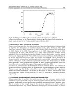
Considerable concern has been raised about the use of a universal, simple relationship, as specified under IPCC Tier 1, in GHG
emissions calculations for biofuels [37]. This is largely because of the possibility of substantially underestimating the release of N2O
associated with the application of artificial N fertilizers and other sources of N in biomass feedstock cultivation. Hence, this issue is
currently under further investigation. However, in the absence of any broadly accepted and agreed alternative, the IPCC Tier 1
approach is commonly applied in GHG emissions calculations. In some instances, the IPCC Tier 1 approach is used selectively, as
there is uncertainty about the reliability of the evaluation of indirect N2O emissions from leaching and runoff, for example. The
actual mechanisms involved in determining total N2O emissions from soil are clearly complex and depend on many specific

considerations. In contrast, the IPCC Tier 1 approach is intentionally simple and, it must be recalled, was derived for application in
the generation of national GHG emissions inventories rather than, particularly, biofuel regulation. To a certain degree, uncertainty is
reflected in the wide variation in the IPCC Tier 1 default values for soil N2O emissions. For example, the simple relationship
produces an average emissions factor of 0.0208 kg N2O kg−1 N, whereas the full range, which reflects the best and worst combina­
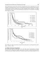
tion of default values, extends from 0.0091 to 0.0527 kg N2O kg−1 N. The effect on this variation can have a significant impact on the
net GHG emissions savings of certain biofuels, as illustrated in Figure 6. In particular, it can be seen that bioethanol production


122

Issues, Constraints & Limitations

70
Net GHG emissions savings (%)

Bioethanol from wheat grain; UK (a)
60
Bioethanol from sugar beet; UK (a)

50
40

Bioethanol from maize/corn; USA (a)

30

Biodiesel from oilseed rape; UK (a)

20

Biodiesel from sunflowers; France (a)

10
Biodiesel from soybean; USA (a)
0
0

0.01

0.02

0.03

0.04

0.05

0.06

Soil nitrous oxide emissions factor (kg N2O/kg−1 N)
Figure 6 Variation of net greenhouse gas (GHG) emissions savings for current biofuels with soil nitrous oxide emissions from artificial nitrogen fertilizer
application. Note: (a) Processing with a natural gas-fired combined heat and power unit.

from UK wheat grain and US maize/corn and biodiesel production from French sunflowers and UK oilseed rape are all adversely
affected by the assumed soil N2O emissions factor.
Hence, improvements in the evaluation of soil N2O emissions for a number of current biofuels are an urgent priority.
Fundamental work in this area has been initiated to derive a more reliable approach to estimating soil N2O emissions and, if
possible, to reduce them. For example, in the United Kingdom, a major research study, referred to as the MIN-NO project, funded by
the Department for Environment, Food and Rural Affairs and the Scottish Government, is undertaking field measurements and
these will be used with the DNDC model to generate, if necessary, a more representative relationship between N fertilizer

application rates and soil N2O emissions [38]. This study is planned to report final results in 2014. Other studies have focused
on specific aspects of the issue and the potential effects of particular mitigation measures. A review of existing knowledge and its
implications for current biofuels was conducted for the RFA during 2009 [21]. From this and other work, it is apparent that any
future evaluation of soil N2O emissions will have to take into account a number of very specific factors including the nature of the
soil, the details of cultivation, the form of artificial N fertilizer, and the type of weather following application. In particular, it
appears that the timing of fertilizer applications and the possibility of soil waterlogging are important considerations. Hence, a more
reliable and representative approach to evaluation may well be a complex procedure rather than a simple relationship. This could
affect the possibility of generating soil N2O emission default value maps or atlases which would, ideally, be very helpful for
estimating GHG emissions for biofuel production.
In addition to these complexities, there are other aspects that may need to be taken into account. Among these is whether soil
N2O emissions from the incorporation of crop residues and the application of organic manures and composts should be included in
GHG emissions calculations for biofuels. Currently, standard calculators promoted by the EC and national regulators do not seem
to include these sources of N2O emissions (see, e.g., References [39–41]). Previously, the issue of crop residue incorporation has
been addressed in GHG emissions calculation only through adjustments for possible effects on the artificial fertilizer requirements
of following crops. However, a clear approach to this based on sound evidence has not been devised. Hence, this is normally
excluded from most GHG emissions calculations. However, it is possible to account for effects of crop residue incorporation using
IPCC Tier 1 default values [26] and assumptions concerning the N content of the residues and the amount incorporated. It should
be noted that the removal of some of these residues for other purposes, obviously, reduces any soil N2O emissions attributed to
the biofuel.
The consequences for soil N2O emissions of applying organic manures have also been discounted previously in GHG emissions
calculations for biofuels. When explicit, the justification for this was that these are attributed to the livestock that originally
produced them, as they would not exist otherwise. The only GHG emissions accounted for have been those associated with the
actual process of applying these manures. However, a counterargument is that these manures provide N for the biofuel crop and this
reduces the need for artificial N fertilizer. Hence, related soil N2O emissions should be taken into account. Again, this can be
achieved using IPCC Tier 1 default values [26], standard data on the N content of various manures (see, e.g., Reference 42), and
assumptions about N losses during storage prior to application. In the context of this last point, it seems to be reasoned that N losses
during storage, leading to N2O emissions, are attributed to the livestock from which they originated.
A further consideration related to the soil N2O emissions from the incorporation of crop residues and the application of organic
manures and composts is that such activities can introduce and maintain carbon in the soil. Hence, it can also be argued that this is a
beneficial effect that, under certain circumstances, results in a degree of carbon sequestration, which should also be accounted for, as

a ‘credit’, in GHG emissions calculations. This argument might seem to find some possible traction within the details of the EC
Renewable Directive [4] and treatment of carbon stocks in relation to dLUC [25]. However, the acceptance of this approach depends


Life Cycle Analysis Perspective on Greenhouse Gas Savings

123

on the level of carbon sequestration that might be achieved and how evidence might be collected and reported to support this. It
should be noted that there is current scientific debate over levels of carbon sequestration, which are affected by the type of soil, its
past history, and any ongoing buildup or saturation of carbon. Additionally, while carbon sequestration accredited to the biofuel
crop might be justified through the incorporation of its residues, there is potential disagreement concerning whether any benefits
from organic manure application can be regarded in the same way. It has been argued that any carbon sequestration cannot be
attributed to a crop treated with organic manures since this really involves moving carbon from one place (where the livestock
obtained their food) to another (where the treated crop is grown). The reason why considerations about possible carbon
sequestration are important is that the estimated carbon credit can counterbalance the negative impacts of related soil N2O
emission. These issues require detailed scientific investigation and sound evidence for their resolution in terms of GHG emissions
calculations for biofuels.
Another issue related to soil N2O emissions is the contribution made to total GHG emissions from the manufacture of artificial
N fertilizers. This contribution can be significant for certain current biofuels, as shown previously in Figure 3. The GHG emissions
factor for an artificial N fertilizer depends on the type of fertilizer and the nature of the technology used in its manufacture. The most
common forms of artificial N fertilizers are ammonium nitrate and urea. As summarized in Table 5, there are a number of different
estimates for the GHG emissions factors of these forms of fertilizer. Two particular features will be seen in Table 5. The first is that
the GHG emissions factors for urea are substantially less than those for ammonium nitrate. From this, it might be concluded that,
from a GHG emissions perspective, it would be advantageous to use urea instead of ammonium nitrate. However, leaving aside
differences in the suitability of these particular N fertilizers and their take-up by certain crops in specific situations, the overall
benefits of this potential switch are less obvious in terms of total GHG emissions, which reflect both artificial N fertilizer
manufacture and application [45]. This is because urea application generates soil CO2 emissions as well as N2O emissions.
Additionally, lime may also have to be applied to counteract possible acidification effects of urea application, resulting in GHG
emissions from both lime manufacture and related soil CO2 emissions. Furthermore, it has been suggested that there are differences

in soil N2O emissions caused by different forms of artificial N fertilizers [46]. The second feature apparent in Table 5 is that there is a
significant difference in the GHG emissions factor for ammonium nitrate manufacture between average production and best
available technology (BAT). It is generally expected that, in the European Union at least, the fertilizer manufacturing industry will
move quickly toward BAT as a result of involvement in the European Union Emissions Trading Scheme. Hence, the GHG emissions
factors for BAT are likely to be more relevant in GHG emissions calculations in the foreseeable future. The possible effect of this on
the net GHG emissions savings of current biofuels is demonstrated in Figure 7. It will be seen that there are marked improvements
in the net GHG emissions savings of specific biofuels, for example, biodiesel production from UK oilseed rape.

5.09.9 Sources of Processing Energy
Another factor that influences the net GHG emissions savings of biofuels is the source of energy normally used to provide heat and
electricity in the conversion process. Various sources of heat and electricity can be adopted and illustrations of their effects on net
GHG emissions savings are provided for bioethanol and biodiesel in Figures 8 and 9, respectively. The options chosen for these
illustrations consist of providing heat by means of coal-, oil-, natural gas-, straw-, and wood-fired boilers with electricity derived
from the relevant national grid in each case and also from coal-, oil-, natural gas-, straw-, and wood-fired CHP units. A number of

Table 5

Selection of greenhouse gas emissions factors for ammonium nitrate and urea fertilizer manufacture
Emissions factor

Form of artificial nitrogen
fertilizer
Ammonium nitrate
NNFCC databaseb
BIOGRACE databasec
EFMA EU 2006d
EFMA EU BATe
Urea
EFMA EU 2006d
EFAM EU BATe

Carbon dioxide
emissions (kg
CO2 kg−1 N))

Methane emissions
(kg CH4 kg−1 N)

Nitrous oxide emissions
(kg N2O kg−1 N)

Total greenhouse gas
emissionsa (kg eq. CO2 kg−1 N)

2.245
2.827
2.343
1.771

0.0121
0.0087
0.0062
0.0050

0.0147
0.0096
0.0125
0.0028

6.875

5.869
6.186
2.715

1.391
0.978

0.0076
0.0066

0
0

1.568
1.130

Using global warming potentials of 23 kg eq. CO2 kg−1 CH4 and 296 kg eq. CO2 kg−1 N2O from the IPCC Third Assessment Report [10] as consistent with the EC Renewable Energy

Directive [4].

b
Average production in Western Europe [43].

c
BIOGRACE list of standard values [44].

d
European Union’s average value for 2006 [45].

e

European Union’s best available technology [45].

a


124

Issues, Constraints & Limitations

68

70

Net GHG emissions savings (%)

60

65

63

65
61

56
50

48

50

49
47

40

39

40

N fertilizer GHG factor:
current default value

30
N fertilizer GHG factor:
BAT today value

20
10
0
Bioethanol Bioethanol Bioethanol
Biodiesel
Biodiesel
from wheat from sugar
from
from oilseed
from
grain; UK (a) beet; UK (a) maize/corn; rape; UK (a) sunflowers;
USA (a)
France (a)

Biodiesel
from
soybean;
USA (a)

Figure 7 Variation of net greenhouse gas (GHG) emissions savings for current biofuels with total GHG emissions from ammonium nitrate fertilizer
manufacture. Note: (a) Processing with a natural gas-fired combined heat and power unit.

39
43

Coal-fired boiler and
grid electricity

46
53
55
59
57
56
60
59

Bioethanol from UK wheat grain

Oil-fired boiler and
grid electricity
Natural gas-fired boiler and
grid electricity

25
36

Straw-fired boiler and
grid electricity

45
66
71
67
67

Bioethanol from UK sugar beet
63

Wood-fired boiler and
grid electricity
Coal-fired CHP unit
81
81
Oil-fired CHP unit

8

20

39

52

Bioethanol from US maize/corn

Natural Gas-fired CHP unit
58

74

61

Straw-fired CHP unit

67
71
68

0

10

20

30

40

50

60

70

Wood-fired CHP unit
80

90

100

Net greenhouse emissions savings (%)
Figure 8 Net greenhouse gas emissions savings of bioethanol with different sources of processing energy. CHP, combined heat and power.

important features are apparent in these illustrations. Probably the most obvious is that there are differences in the net GHG
emissions savings for either bioethanol or biodiesel production from different biomass feedstocks using the same source of
processing energy, in the form of either a boiler with grid electricity or CHP. As already discussed, this is mainly due to differences
in GHG emissions associated with the provision of the original biomass feedstocks. However, some differences can arise in


Life Cycle Analysis Perspective on Greenhouse Gas Savings

28
30
32
36
37
43
41
39
40
39

Biodiesel from UK oilseed rape

36
37
38
41
42

Biodiesel from US soybean

49
48
47
46
45

37
38
39
40
41
40
40
40
41
41

Bioethanol from French sunflowers

0

125

Coal-fired boiler and grid electricity
Oil-fired boiler and grid electricity
Natural gas-fired boiler and grid electricity
Straw-fired boiler and grid electricity
Wood-fired boiler and grid electricity
Coal-fired CHP unit
Oil-fired CHP unit
Natural gas-fired CHP unit
Straw-fired CHP unit
Wood-fired CHP unit

10 20 30 40 50 60 70 80 90 100
Net greenhouse emissions savings (%)

Figure 9 Net greenhouse gas emissions savings of biodiesel with different sources of processing energy. CHP, combined heat and power.

processing for the same biofuel, which, for example, result from different fermentation dynamics for different biomass feedstocks.
Furthermore, in cases where grid electricity is used, national differences in GHG emissions factors have to be taken into account.
Such considerations can be relatively minor compared with differences between the sources of processing energy used to derive a
given biofuel from each specific biomass feedstock. In particular, due to their greater overall energy efficiency, the use of CHP units,
generally, results in higher net GHG emissions savings than with the use of a separate boiler and grid electricity. Comparisons are, of
course, affected by whether the basic source of fuel in the CHP plant and boiler is a fossil fuel or a biomass fuel. However, the effect
of this may be less pronounced than might, at first, be expected. This is primarily a consequence of applying the EC Renewable
Energy Directive methodology for GHG emissions calculations to the specific treatment of surplus electricity generated by CHP
units and sold to the grid. In many situations, including most biofuel production plants, CHP units are principally designed to meet
process heat requirements. These are often quite large while the process electricity requirements are relatively small. Hence,

depending on particular circumstances, the CHP unit has surplus electricity, which can be exported to the grid, thereby improving
the overall economics of the process.
With the EC Renewable Energy Directive methodology, such surplus CHP electricity is accounted for in GHG emissions
calculations by means of a substitution credit. However, unlike some methodologies that base this credit on the GHG emissions
factor for grid electricity, the EC Renewable Energy Directive adopts a quite different approach. This involves establishing a credit
based on a GHG emissions factor of a power-only unit using the same fuel as the CHP unit. It appears that the justification for this
somewhat convoluted approach is to account for alternative uses of any given fuel. If such is the justification, then it would seem the
methodology is attempting, incorrectly, to address both regulatory and policy analysis objectives simultaneously. Be this as it may,
the overall effect of this particular approach within the EC Renewable Energy Directive is that the substitution credits for surplus
electricity from biomass-fired CHP units is lower than those associated with fossil fuel-fired CHP units. Of course, there are direct
benefits, in terms of reduced GHG emissions, from the operation of biomass-fired CHP units, but these can be moderated by
reduced indirect benefits from surplus electricity sales.
The overall effect of this is demonstrated in Figure 10, which shows the net GHG emissions savings from bioethanol produced
using CHP from UK wheat grain with different emissions factors for surplus electricity. In this particular case, the surplus electricity
from the CHP unit is relatively high at 642 kWh per tonne of bioethanol. With a natural gas-fired CHP unit, the resulting credit
based on the EC Renewable Energy Directive equates to 12% of the total GHG emissions. In Figure 10, net GHG emissions savings
are compared for those using the approach of the EC Renewable Energy Directive and those with a credit based on UK grid electricity
in 2006 equal to 0.581 kg eq. CO2 kWh−1. With a coal-fired CHP unit, the net GHG emissions savings decrease when a grid
electricity credit is used. There is no significant change for an oil-fired CHP unit. However, in the case of natural gas-, straw-, and
wood-fired CHP units, the net GHG emissions savings all increase. This is most pronounced for biomass-fired CHP units.
Figure 10 demonstrates that by adopting equivalent sourced electricity for surplus CHP electricity within the provisions of the
EC Renewable Energy Directive, differences in net GHG emissions savings are relatively limited, ranging between 56% and 60% for
fossil fuel- and biomass-fired CHP units used in the production of bioethanol from UK wheat grain. However, if UK grid electricity
is displaced, differences are somewhat enhanced, ranging from 54% for coal-fired CHP to 67% for wood-fired CHP. This would
seem to reflect, more realistically, the advantages of biomass-fired CHP units in terms of GHG emissions savings. Indeed, this
approach is more relevant as it communicates the benefits of such CHP units to the economic operators who decide the sources of


126

Issues, Constraints & Limitations

Coal-fired CHP unit: displacement of equivalent sourced electricity
Coal-fired CHP unit: displacement of UK grid electricity
Oil-fired CHP unit: displacement of equivalent sourced electricity

59
54

Oil-fired CHP unit: displacement of UK grid electricity

57
Natural gas-fired CHP unit: displacement of equivalent sourced electricity

57
56

Natural gas-fired CHP unit: displacement of UK grid electricity

59
Straw-fired CHP unit: displacement of equivalent sourced electricity

60
66

Straw-fired CHP unit: displacement of UK grid electricity

59

Wood-fired CHP unit: displacement of equivalent seourced electricity

67

Wood-fired CHP unit: displacement of UK grid electricity
0

10

20

30

40

50

60

70

80

90 100

Net greenhouse emissions savings (%)
Figure 10 Effect of emissions factor for surplus electricity credit on net emissions savings for bioethanol from UK wheat grain. CHP, combined heat and
power.

processing energy for biofuel plants. However, adopting the current approach specified in the EC Renewable Energy Directive could,
perversely, discourage the use of biomass-fired CHP units. This is particularly the case when differences in net GHG emissions

savings between biofuel production using biomass-fired and fossil fuel-fired CHP units are relatively small, and the economics of
the former is significantly less favorable relative to the latter.

5.09.10 Coproducts
The production of many current biofuels generates other products, referred to as coproducts or by-products depending mainly on
their economic significance. These other products have to be taken into account in the calculation of GHG emissions. As discussed
previously, this is achieved through the application of allocation procedures, which, as the phrase suggests, is an attempt to share
GHG emissions between all the products that emerge from any given process. However, among all the possible allocation
procedures proposed, one method does not strictly comply with the concept of ‘sharing’ GHG emissions. This allocation procedure
consists of using substitution credits for all coproducts apart from the main product. With this particular procedure substitution
credits are subtracted from the total GHG emissions process. As such, the use of substitution credits is an accounting mechanism
rather an allocation procedure. As explained previously, the use of substitution credits complies with consequential LCA, which is
relevant to policy analysis. In contrast, true allocation procedures reflect attributional LCA, which is necessary for regulation.
Leaving aside the fundamental differences and relevance of allocation procedures, it has been suggested that their application
has no significant effect on the estimated net GHG emissions savings of biofuels. For example, in justification of its use of coproduct
allocation based on energy content, it is stated in the EC Renewable Energy Directive that
The substitution method is appropriate for the purposes of policy analysis, but not for the regulation of individual economic operators and individual
consignments of transport fuels. In those cases, the energy allocation method is the most appropriate method, as it is easy to apply, is predictable over time,
minimises counter-productive incentives and produces results that are generally comparable with those produced by the substitution method [4, para 81, p. 18].

However, as demonstrated in Figure 11, this last aspect is not necessarily correct. Figure 11 summarizes the net GHG emissions
savings of current biofuels using coproduct allocation by energy content, mass, price, and substitution credits. Apart from these
differences in allocation procedures, these results are based on the same assumptions as those shown previously for these particular
biofuels. Very substantial differences in net GHG emissions savings are apparent for some biofuels, especially between allocation by
energy content and adoption of substitution credits.
The essential details of the substitution credits used to generate the results shown in Figure 11 are summarized in Table 6.
Various considerations affect the detailed application of substitution credits in GHG emissions calculations. In particular, it is
necessary to identify the specific product that the coproduct under consideration is expected to displace, its means of production,
and, therefore, its emission factor. There are many possible options for displacement and the choice needs to be appropriate for the
specific context of the policy analysis that is being undertaken. This determines the realistic alternatives and the timescales in

question. It is also necessary to determine the ‘equivalence’ of the coproduct to the displaced product because one may not be an


Life Cycle Analysis Perspective on Greenhouse Gas Savings

127

39
Biodiesel from UK oilseed rape (a)

72

16
12
47

Biodiesel from US soybean (a)

68

51
50
40

Biodiesel from French sunflowers (a)

60

10
32

82
83
80

Biodiesel from UK recycled vegetable oil (b)

88
56
Bioethanol from UK wheat grain (a)

63

35
46

63
Bioethanol from UK sugar beet (a)

60

24

69

61
Bioethanol from US maize/corn (a)

45
0

10

20

30

40

50

68
50
60

70

80

90 100

Net greenhouse gas emissions savings (%)
Energy content allocation

Mass allocation

Price allocation

Substitution credits

Figure 11 Effect of coproduct allocation procedures on net greenhouse gas emissions savings of current biofuels. Notes: (a) Processing with a natural
gas-fired combined heat and power unit. (b) Processing with a natural gas-fired boiler and grid electricity.

exact replacement of the other. This requires a meaningful basis for comparing alternative products. For example, for coproducts
that are animal feeds, calorific value, protein content, digestibility, etc., may feature separately or in combination when establishing
equivalence as part of GHG emissions calculations. Finally, any extra processing of coproducts has to be taken into account when
using substitution credits in GHG emissions calculations. This is because comparisons are, in effect, being made between finished
products. Hence, in the case of animal feeds, drying to an equivalent moisture content has to be included. This contrasts with the
approach adopted in other allocation procedures that do not need to take into account any GHG emissions associated with a
coproduct once it has been separated from the main product. These and other considerations mean that the net GHG emissions for
biofuels determined using substitution credits can vary substantially depending on the basic assumptions incorporated into the
calculations. These assumptions should reflect the nature of the policy analysis that is being conducted and, as such, should be
stated clearly and comprehensively when results are quoted. The appropriate approach to such analysis needs to incorporate global
modeling, similar to that necessary to address the effects of iLUC, in order to accommodate the dynamic and interactive
consequences of product displacement and substitution.

5.09.11 Future Biofuel Technologies
In addition to current biofuels, there are a number of new technologies under development and commercialization that have the
potential to avoid some of their negative impacts, in terms of GHG emissions. These future biofuel technologies often involve the
utilization of different and, in some cases, novel biomass feedstocks and advanced conversion techniques that do not rely on
fermentation or esterification. Many of the possible biomass feedstocks enable the impacts of dLUC, iLUC, and soil N2O emissions
to be reduced, by using nonfood crops that can achieve higher yields than conventional crops required for current biofuels. Such
biomass feedstocks include cultivated sources of wood, such as short-rotation coppice (SRC), short-rotation forest (SRF) and
conventional forests, and grasses, such as reed canary grass, miscanthus, and switchgrass. Other possible biomass feedstocks offer
the opportunity to avoid the impacts of dLUC, iLUC, and soil N2O emissions completely by using noncrop sources, such as
agricultural residues, wood wastes, other waste products and municipal solid waste (MSW), and novel sources such as algae. The
potential utilization of these types of biomass feedstocks for biofuel production is not without some important implications and
considerations, however. For example, land availability may constrain the cultivation of nonfood crops. Additionally, the avail­
ability of residues and wastes is governed by factors other than the demand for biofuels and they may have significant competing

128

Issues, Constraints & Limitations

Table 6

Summary of substitution credits for coproduct allocation

Biofuel and coproduct
Biodiesel production from UK oilseed rape
Rape meal
Glycerin
Biodiesel production from US soybean
Soy meal
Glycerin
Biodiesel production from French sunflowers
Sunflower meal
Glycerin
Biodiesel production from UK recycled vegetable oil
Glycerin
Bioethanol production from UK wheat grain
Distillers’ dark grains and solubles
Bioethanol production from UK sugar beet
Beet pulp
Bioethanol production from US maize/corn
Distillers’ dark grains and solubles

Coproduct output
(tonne coproduct

per tonne biofuel)

Substitution credit
(kg eq. CO2
per tonne coproduct)

1.58
0.20

504a
2170b

3.76
0.15

373c
2170b

0.45
0.15

504a
2170b

0.20

2170b

1.14

491d

1.25

337e

0.93

283f

a

Based on displacement of soy meal from soybeans grown in the United States and milled in the United Kingdom and a substitution credit of 504 kg

eq. CO2 per tonne rape or sunflower meal [3]. This can be compared with displacement of 0.80 t soy meal per tonne rape meal and an emissions factor

for US soy meal imported into the European Union of 65 kg eq. CO2 per tonne soy meal [47].

b
Based on an emissions factor for propylene glycol of 2170 kg eq. CO2 per tonne [47].

c
Based on displacement of wheat grain grown in the European Union and a substitution credit of 373 kg eq. CO2 per tonne soy meal [3].

d
Based on displacement of soy meal from soybeans grown in the United States and milled in the United Kingdom and a substitution credit of 491 kg

eq. CO2 per tonne distillers’ dark grains and solubles [3]. This can be compared with displacement of 0.78 t soy meal per tonne distillers’ dark grains

and solubles and an emissions factor for US soy meal imported into the European Union of 65 kg eq. CO2 per tonne soy meal [47].

e
Based on displacement of UK wheat grain and a substitution credit of 337 kg eq. CO2 per tonne beet pulp [3].

f
Based on displacement of US corn gluten feed and a substitution credit of 283 kg eq. CO2 per tonne distillers’ dark grains and solubles [3].


applications. The utilization of all these sources depends on new processing technologies that can extract suitable materials in
sufficient quantities from biomass and convert them into suitable biofuels. In some cases, instead of extracting and processing oils,
starches, or sugars, these new technologies exploit abundant lignocellulosic material either by means of enzymes or through
gasification, as in Fischer–Tropsch processing, to obtain biofuels such as syndiesel and, with biomethanization, bioSNG. In the case
of algae, it may be possible to extract natural oils directly and convert them into suitable biofuels.
Future biofuel technologies are at various stages of development and commercialization. Hence, it is not possible to
establish definitive estimates of their net GHG emissions savings since, realistically, this requires basic, proven information
on the actual provision of relevant biomass feedstocks and on the actual performance of conversion techniques. However,
indicative estimates of net GHG emissions savings, based on proposed or speculative data for future biofuel technologies, can be
derived. An example of this is illustrated in Figure 12, which presents estimated net GHG emissions savings for the production
of syndiesel and bioSNG from a variety of biomass feedstocks using the methodology of the EC Renewable Energy Directive
[13, 15]. In general, Figure 12 indicates the potential to achieve very high net GHG emissions savings. However, this requires
some qualification. In particular, it should be noted that any impacts of dLUC and iLUC have not been incorporated in these
estimates. Depending on the actual choices in sourcing specific biomass feedstocks, this could affect the net GHG emissions
savings for syndiesel and bioSNG derived from SRC, SRF, timber, miscanthus, and switchgrass. Although high net GHG
emissions savings are indicated for most residues and wastes, some, such as those for syndiesel and bioSNG derived from
straw and MSW, are noticeably lower. This is due to the combination of relatively low net calorific values for these biomass
feedstocks and the GHG emissions associated with their provision consisting of collecting, baling, and transporting, in the case
of straw, and pelletizing, in the case of MSW.
The results presented in Figure 12 are based on the GHG emissions calculation methodology of the EC Renewable Energy
Directive which excludes the effect of so-called reference systems. This is appropriate for calculations that are used for regulatory
purposes and, hence, are based on attributional LCA. However, in the context of policy analysis which requires the application

of consequential LCA, the overall or global impacts of an activity have to be taken into account. This involves establishing reference
systems that determine the GHG emissions implication of the chains of consequences that an activity initiates, in the same way
that the impacts of iLUC have to be addressed. However, unlike most of the effects of iLUC, sometimes activities can promote
positive consequences, such as the avoidance of GHG emissions. Such is the case when considering the use of wastes in biofuel
production. In such instances, the need to dispose of wastes means that significant GHG emissions can be avoided. The importance
of this, from a policy analysis perspective, is illustrated in Figure 13, which shows estimated net GHG emissions for syndiesel and
bioSNG generated from a selection of wastes without and with the effect of reference systems [13, 15]. In this instance, it has been


129

Life Cycle Analysis Perspective on Greenhouse Gas Savings

BioSNG from UK switchgrass bales
BioSNG from UK miscanthus bales
BioSNG from UK miscanthus chips
BioSNG from UK short-rotation coppice wood chips
BioSNG from UK short-rotation forest wood chips
BioSNG from UK timber wood chips
BioSNG from UK straw bales
BioSNG from UK municipal solid waste pellets
BioSNG from UK commercial cardboard waste pellets
BioSNG from UK aboricultural arisings wood chips
BioSNG from UK forestry residue wood chips
BioSNG from UK pallet and demolition waste wood chips
BioSNG from UK clean waste wood chips
Syndiesel from UK switchgrass bales
Syndiesel from UK miscanthus bales
Syndiesel from UK miscanthus chips
Syndiesel from UK short-rotation coppice wood chips

Syndiesel from UK short-rotation forest wood chips
Syndiesel from UK timber wood chips
Syndiesel from UK straw bales
Syndiesel from UK municipal solid waste pellets
Syndiesel from UK commercial cardboard waste pellets
Syndiesel from UK forestry residue wood chips
Syndiesel from UK pallet and demolition waste wood chips
Syndiesel from UK clean waste wood chips

87
88
88
91
91
92
80
74
92
93
93
94
94
86
88
88
94
94
95
73
61

95
98
99
99
0

10

20

30

40

50

60

70

80

90

100

Net greenhouse gas emissions savings (%)
Figure 12 Net greenhouse gas emissions savings for some future biofuels. BioSNG, biosynthetic natural gas.

74

BioSNG from UK municipal solid waste pellets

123
92

BioSNG from UK commercial cardboard waste pellets

217
94

BioSNG from UK pallet and demolition waste wood chips

237
94

BioSNG from UK clean waste wood chips

221
61

Syndiesel from UK municipal solid waste pellets

153
95

Syndiesel from UK commercial cardboard waste pellets

327
99

Syndiesel from UK pallet and demolition waste wood chips

361
99

Syndiesel from UK clean waste wood chips

332
0

50
100
150
200
250
300
350
Net greenhouse gas emissions savings (%)
Without reference system

400

With reference system

Figure 13 Net greenhouse gas emissions savings for future biofuels from wastes without and with reference systems. BioSNG, biosynthetic natural gas.

assumed that the alternative to biofuel production is disposal to landfill with subsequent methane capture and electricity
generation, which, subsequently, displaces national grid supplies. The effect of this is to moderate the GHG emissions benefits
compared with simple disposal to landfill. Figure 13 demonstrates that, by taking the reference system into account, net GHG

emissions savings can exceed 100%.


130

Issues, Constraints & Limitations

5.09.12 Conclusions and Recommendations
It has been shown that there are many factors that can influence the evaluation of total GHG emissions and net GHG emissions
savings for biofuels. These can cause small or large differences in results. They can also combine together to generate a considerable
range of results for any particular biofuel. Hence, it is absolutely essential to qualify any results with the basic assumptions that have
been made about the details of the biofuel, its biomass feedstock, how this is obtained, processed, and converted, and, crucially, the
GHG emissions calculation methodology adopted and, ultimately, the reasons behind the generation of results. In the currently
contentious debate surrounding biofuels, it is vital that such matters are clearly stated and that adequate transparency is displayed in
the publication of results. Ideally, this means that all details of GHG emissions calculations should be made available within the
accepted constraints of commercial confidentiality.
However, the issue of potential variations in results is not simply an academic concern. Even small changes in results can be very
important when set in the context of specific targets for net GHG emissions savings for commercially produced biofuels. For
example, the EC Renewable Energy Directive specifies minimum net GHG emissions savings of 35% for current biofuels supplied in
the European Union, rising to 50% from 1 January 2017, with a target of at least 60% for biofuels and bioliquids produced from
plants starting production on or after 1 January 2017 [4]. From the results illustrated here, it can be seen that a change or
combination of changes in the specific details of the production of a biofuel could make a significant difference on whether it
complies with current or future net GHG emissions savings targets.
Such sensitivity also explains why there is concern among commercial biofuel producers over the possibility of modifying
existing GHG emissions calculations and net GHG emissions savings targets in the light of further scientific knowledge, especially
regarding the effects of iLUC and, to a lesser degree, soil N2O emissions. To an economic operator, this introduces considerable
policy risk into an already demanding decision-making process that includes both technology and financial risk. While it is
necessary to ensure that biofuels provide positive benefits in terms of GHG emissions mitigation, it is important to realize that
targets for the supply of biofuels will not be achieved without substantial commitment and investment by such economic operators.
This does not mean that new scientific understanding should be ignored. Instead, uncertainty should be reduced by appreciating

the distinction between the fundamental purposes, principles, and application of attributional and consequential LCA. Hence, in
the regulation of biofuel producers with respect to the declared net GHG emissions savings of their products, attributional LCA
should be applied, rigorously and consistently. One particular result of the strict application of the logic of attributional LCA is that
the evaluation of net GHG emissions savings from biofuels for regulatory purposes should exclude the effects of iLUC as these are
well outside the control or clear influence of economic operators. However, evaluation of the effects of iLUC is obviously and
legitimately within the scope of policy analysis which sets the targets for levels of biofuel production. Such matters are most
appropriately addressed by consequential LCA.
In addition to these fundamental issues, the further development and implementation of biofuels will depend on a number of
important considerations, which include
• ‘low-carbon’ biomass feedstock cultivation techniques such as enhancing crop yields without increasing nitrogen fertilizer
application rates,
• advanced biofuel processing technologies that can increase overall conversion efficiencies and utilize a wider range of biomass
feedstocks,
• improved scientific knowledge concerning the effect of dLUC and soil N2O emissions,
• agreement on the effects of iLUC through establishment of reliable global land use change modeling,
• international harmonization of appropriate GHG emission calculation methodologies and their relevant databases, and
• application of robust and widespread certification procedures that support GHG emissions calculations for regulatory purposes
[48, 49].

References
[1] ISO (1999) Environmental management – life cycle assessment – goal and scope definition and inventory analysis. BS EN ISO 14041. London, UK: British Standards
Institute.
[2] ISO (2006) Environmental management – life cycle assessment – principles and framework. BS EN ISO 14040. London, UK: British Standards Institute.
[3] RFA (2009) Carbon and sustainability reporting within the renewable transport fuel obligation: Technical guidance parts 1 and 2, version 2.0. St. Leonards-on-Sea, UK:
Renewable Fuels Agency. (accessed March 2009).
[4] EC (2009) Directive 2009/28/EC of the European parliament and of the council of 23 April 2009 on the promotion of the use of energy from renewable sources and amending
and subsequently repealing directives 2001/77/EC and 2003/30/EC. Brussels Belgium: European Commission.
[5] BSI (2008) PAS 2050 – specification for the assessment of life cycle greenhouse gas emissions of goods and services. Publicly Available Specification. London, UK: British
Standards Institution, October 2008.
[6] DEFRA (2008) Biomass environmental assessment tool, version 2.0. Prepared by AEA Group plc and North Energy Associates Ltd for Department for Environment, Food and

Rural Affairs and the Environment Agency, London, UK. (accessed November 2008).
[7] RFA (2010) Carbon and sustainability reporting within the renewable transport fuel obligation: Technical guidance parts 1 and 2, version 3.2. St. Leonards-on-Sea, UK:
Renewable Fuels Agency. (accessed April 2010).


Life Cycle Analysis Perspective on Greenhouse Gas Savings

131

[8] Brander MT, Hutchinson C, and Davis G (2009) Consequential and attributional approaches to LCA: A guide to policy makers with specific reference to greenhouse gas LCA of
biofuels. Technical Paper TP-090403-A. Edinburgh, UK: Ecometrica Press. (accessed April 2009).
[9] IPCC (1996) Climate change 1995: Second assessment report of the IPCC. Intergovernmental Panel on Climate Change. Cambridge University Press, Cambridge. c.
ch/ipccreports/assessment-reports.php (last accessed 7 December 2009).
[10] IPCC (2001) Climate change 2001: The scientific basis; Contribution of working group 1 to the third assessment report of the IPCC. Intergovernmental Panel on Climate
Change. Cambridge, UK: Cambridge University Press. (last accessed 7 December 2007).
[11] IPCC (2007) Climate change 2007: Synthesis report: Fourth assessment report. Intergovernmental Panel on Climate Change. Cambridge University Press, Cambridge.
(last accessed 7 December 2009).
[12] Hill N, Mortimer ND, Bates J, et al. (2008) Implementation of the EU biomass action plan and the biofuel strategy: Comparing GHG emission reduction performance of different
bio-energy applications on a life cycle basis. Brussels, Belgium: AEA Technology plc for the Directorate-General for the Environment, European Commission.
[13] Mortimer ND, Evans AKF, Shaw VL, and Hunter AJ (2009) Life cycle and techno-economic assessment of the north east biomass to liquids project. Contract No. 08/016. York,
UK: North Energy Associates Ltd for the National Non-Food Crops Centre. (accessed February 2009).
[14] Mortimer ND, Evans AKF, Ashley A, et al. (2010) Comparison of the greenhouse gas benefits resulting from use of vegetable oils for electricity, heat, transport and industrial
purposes. Project Code NNFCC10-016. York, UK: North Energy Associates Ltd for the Department for Energy and Climate Change via the National Non-Food Crops Centre.
(accessed February 2010).
[15] Mortimer ND, Evans AKF, Mwabonje O, et al. (2010) Analysis of the greenhouse gas emissions for thermochemical BioSNG production and use in the United Kingdom. Project
Code NNFCC10-009. York, UK: North Energy Associates Ltd for the National Non-Food Crops Centre. (accessed June 2010).
[16] Dritschilo W, Monroy M, Nash E, et al. (1983) Energy versus food resources ratios for alternative energy technologies. Energy 8(4): 255–265.
[17] Johnson MA (1983) On gasohol and energy analysis. Energy 8(3): 225–233.
[18] Pimental D (2003) Ethanol fuels: Energy balance, economics and environmental impacts are negative. Natural Resources Research 12: 2.
[19] Wang M (1999) GREET 1, version 8a. Chicago, IL: Argonne National Laboratory, University of Chicago.

[20] Mortimer ND (2009) Primary energy and greenhouse gas multipliers for fuels and electricity, United Kingdom 2002. Part of the Statistical Analysis Database for Project NF0614.
York, UK: North Energy Associates Ltd for the Department for Environment, Food and Rural Affairs via the National Non-Food Crops Centre. (accessed
October 2009).
[21] Mortimer ND, Mwabonje O, and Hunter AJ (2009) Nitrous oxide emissions from biofuel feedstock cultivation. St. Leonards-on-Sea, UK: North Energy Associates Ltd for the
Renewable Fuels Agency. (accessed November 2009).
[22] Spirinckx C and Ceuterick D (1996) Comparative Life-Cycle Assessment of Diesel and Biodiesel. Mol, Belgium: VITO (Flemish Institute for Technological Research).
[23] Edwards R, Griesemann J-C, Larivé J-F, and Mahieu V (2003) Well-to-wheels analysis of future automotive fuels and powertrains in the European context: Tank-to-wheels report
(version 1). Ispra, Italy: Institute for Environment and Sustainability, Joint Research Centre.
[24] RFA (2008) The Gallagher review of the indirect effects of biofuel production. St. Leonards-on-Sea, UK: Renewable Fuels Agency.
(accessed July 2008).
[25] EC (2010) Commission decision of 10 June 2010 on guidelines for the calculation of land carbon stocks for the purpose of annex V to directive 2009/28/EC. Official Journal of
the European Union L151: 19–41.
[26] IPCC (2006) IPCC guidelines for national greenhouse gas inventories: Volume 4: Agriculture, forestry and other land use. Edited by Eggleston S, Buendia L, Miwa K, et al.
Kanagawa, Japan: Institute for Global Environmental Strategies. (last accessed 27 May 2008).
[27] EC (2010) Communication from the European Commission on the practical implementation of the EU biofuels and bioliquids sustainability scheme and on counting rules for
biofuels. Official Journal of the European Union C160: 8–16.
[28] Fargione J, Hill J, Tilman D, et al. (2008) Land clearing and the biofuel carbon debt. Science Express. (accessed 7 February 2008).
[29] Searchinger T, Heimlich R, Houghton R, et al. (2008) Use of US croplands for biofuels increases greenhouse gases through emissions from land use change. Science Express
319(5867): 1238–1240.
[30] Bowyer C (2010) Anticipated indirect land use change associated with expanded use of biofuels and bioliquids – an analysis of the national renewable energy action plans.
London, UK: Institute for European Environmental Policy. (accessed November 2010).
[31] Al-Riffai P, Dimaranan B, and Laborde D (2010) Global trade and environmental impact study of the EU biofuels mandate. Washington, DC: ATLASS Consortium, International
Food Policy Institute. (accessed March 2010).
[32] Fonseca MB, Burrell A, Gay H, et al. (2010) Impacts of the EU biofuel target on agricultural markets and land use: A comparative modelling assessment. EUR 24449 EN. Sevilla,
Spain: European Commission Joint Research Centre, Institute for Prospective Technological Studies. />(accessed June 2010).
[33] EC (2010) The impact of land use change on greenhouse gas emissions from biofuels and bioliquids. Brussels, Belgium: Directorate-General for Energy, European
Commission. (accessed July 2010).
[34] Edwards R, Mulligan D, and Marelli L (2010) Indirect land use change from increased biofuels demand: Comparison of models and results for marginal biofuels production from
different feedstocks. EUR 24485 EN. Ispra, Italy: European Commission Joint Research Centre, Institute for Energy. />land_use_change.en.htm (last accessed 14 October 2010).
[35] EC (2010) Report from the commission on indirect land-use change related to biofuels and bioliquids. COM(2010)811 Final. Brussels, Belgium: European Commission.

(accessed 22 December 2010).
[36] UNH (2007) User’s guide for the DNDC model, version 9.1. Durham, NH: Institute for the Study of Earth, Oceans and Space, Complex Systems Research Center, University of
New Hampshire. (accessed 15 April 2007).
[37] Crutzen PJ, Mosier AR, Smith KA, and Winiwarter W (2008) N2O release from agrobiofuel production negates global warming reduction by replacing fossil fuels. Atmospheric
Chemistry and Physics 8: 389–395.
[38] ADAS (2011) Minimising nitrous oxide intensities of arable crop products. LINK Research Project LK09128, ADAS UK Ltd, Boxworth, UK. />Projects/MINNO/tabid/283/Default.aspx (accessed 2 March 2011).
[39] BIOGRACE (2011) Harmonised calculation of biofuel greenhouse gas emissions in Europe: Excel greenhouse gas emission calculation tool; Version 3-public. http://www.
biograce.net (accessed 2 March 2011).
[40] JEC (2011) JEC biofuel pathways RED method; Version 3.0, 14 November 2008. Ispra, Italy: Joint Research Centre-EU CAR-CONCAWE collaboration, Institute for Environment
and Sustainability, European Commission Research Centre. (accessed 2 March 2011).
[41] RFA (2011) RFA_Calculator_RED_Ready_Setup.exe: Carbon calculator RED ready. St. Leonards-on-Sea, UK: Renewable Fuels Agency. .
uk (accessed 2 March 201).
[42] DEFRA (2010) Fertiliser manual: RB209, 8th edn. London, UK: Department for Environment, Food and Rural Affairs. (accessed June 2010).
[43] NNFCC (2009) NF0614NFert02open.xls: Ammonium nitrate production 1996. York, UK: National Non-Food Crops Centre. (accessed 2 March 2011).
[44] BIOGRACE (2011) Harmonised calculation of biofuel greenhouse gas emissions in Europe: List of standard values; Version 2-public. (accessed 2
March 2011).
[45] Brentrup F and Pallière C (2008) GHG emissions and energy efficiency in European nitrogen fertiliser production and use. Proceedings of the International Fertiliser Society, No.
639, York, UK. (Paper presented to International Fertilizer Society at a conference in Cambridge, UK, on 11 December 2008).
[46] Bouwman AF, Boumans LJM, and Batjes NH (2002) Modeling global annual N2O and NO emissions from fertilized fields. Global Biochemical Cycles 16(4): 1–9.


132

Issues, Constraints & Limitations

[47] JEC (2007) Well-to-wheels analysis of future automotive fuels and powertrains in the European context. Well-to-Tank Report, Version 2c, WTT Appendix 1. Ispra, Italy: Institute
for Environment and Sustainability, European Commission Research Centre. (accessed 13 March 2011).
[48] Kindred D, Mortimer N, Sylvester-Bradley R, et al. (2008) Understanding and managing uncertainties to improve biofuel GHG emissions calculations. Project Report No. 435,
Part 2. London, UK: Home Grown Cereals Authority.
[49] Mortimer ND, Ashley A, Evans AKF, et al. (2008) Support for the review of the indirect effects of biofuels. Sheffield, UK: North Energy Associates Ltd for the Renewable Fuels

Agency. (accessed June 2008).