Solution manual cost accounting by LauderbachCONTROL AND EVALUATION OF COST CENTERS
Bạn đang xem bản rút gọn của tài liệu. Xem và tải ngay bản đầy đủ của tài liệu tại đây (100.07 KB, 31 trang )
CHAPTER 11
CONTROL AND EVALUATION OF COST CENTERS
11-1 Outsourcing and Standard Costs
The short life cycle of toys suggests that manufacturers would not
benefit from using standard costs. However, they must bid for
business, which indicates that they examine the toy closely before
setting a price. This analysis is tantamount to developing a standard
cost.
11-2
Responsibility for Variances
1. The material price variance will be favorable, while the material
use, labor efficiency, and VOH efficiency variances will probably be
unfavorable. Quality could also suffer.
2. Before the company changes its standards, we should expect all
efficiency variances to be favorable because of the reduced diversity.
The company might even find material price savings from buying fewer
types of materials and components.
3. The same things we mentioned in part 2 should happen here. Here
the company is reducing complexity of products. Simplification should
result in products that are easier to manufacture.
4. The labor rate variance will be favorable, the labor and variable
overhead efficiency variances probably unfavorable.
11-3
Learning Curves
Auto assembly plants do experience learning effects during
changeovers. Assembly lines run slower for a while, then move up to
full speed as the workers become more familiar with the operations on
the new models. Aircraft plants experience learning effects. The
learning effect was discovered in an aircraft plant in the 1930s. The
others will not show learning effects because they are machine-driven,
processing operations.
11-4
Long-Term Contracts
The principal reasons for using long-term contracts are to ensure
supplies and to obtain firm prices. Many companies willingly sacrifice
the possibility of paying too much (if prices subsequently fall) to
manage the risk of paying too much (if prices rise) or not having an
ensured supply. For Stanley the ensured supply is not a reason because
supplies are available at competitive prices. The price risk is
therefore Stanley’s principal motivation.
The principal disadvantage is the possibility of losing lower
prices in the future. Depending on the terms of the agreement and the
commodity or product, companies might also risk having too great a
supply. If demand for the end product falls and the agreement requires
taking a minimum quantity, the company could have unwanted inventory.
The company might also lose flexibility to substitute other commodities
or products if it is required to take a minimum quantity. Consider the
following statement from Palm’s 2001 Form 10-K.
“Due to supply constrained inventories experienced during the
first three quarters of fiscal year 2001, we built inventory levels for
certain components with long lead times and entered into certain longerterm commitments for certain components. In the fourth quarter, the
sudden and unanticipated significant decrease in demand for our products
caused our inventory levels to exceed our forecasted requirements. We do
not currently anticipate that the excess inventory subject to this
provision will be used at a future date based on our current 12-month
forecast.”
11-5
Productivity Gains
Efficiency variances were favorable (or at least some efficiency
variances were favorable) and at least some price or rate variances were
unfavorable. Increases in productivity typically mean increases in
efficiency. The statement that increased productivity "partially offset
increase in our input costs" indicates that the company paid more for
inputs, which gives rise to rate or price variances.
11-6
Responsibility for Variances
Memorandum
To:
From:
Date:
Subj:
Henry Berger
Student
Today
Identification of rejects
Jack Smith has questioned our allocation of rejects that we cannot
identify by department on the basis of identifiable rejects.
The validity of Smith's claim can neither be verified nor refuted,
given the available information. Obviously, the claim of
discrimination would be valid if the proportions, by department, of
unidentifiable rejects do not equal the proportion of identifiable
rejects. But, by definition, it is impossible to determine the
responsibility for unidentifiable rejects. Hence, Smith's claim can be
neither proved nor disproved. And, from this analysis, it is clear
that we are actually charging managers with an arbitrary allocation:
they are being charged with costs over which they cannot be shown to
have control. This violates the principle of controllability in
responsibility reporting.
One possibility is to stop the allocation entirely, charging the
managers with only the rejects specifically identifiable as having been
caused by their departments. If we were to adopt JIT principles, we
would perform continual inspection, which would eliminate the problem.
Another possibility is to develop new evaluation procedures that can
better identify the sources of rejects. This might require inspecting
after each operation rather than after the total assembly operation is
complete. Even with revised inspection procedures, it might not be
possible to assign all rejects. Moreover, the cost of the new
inspection approach requires justification on the basis that the
benefits to be received will be greater than the cost of the procedure.
11-7
Significance of Variances
Even if total actual costs do not exceed total budgeted costs: (1)
there can be offsetting total variances for individual elements of cost
(materials, labor, individual overhead costs); and (2) a particular
cost element can be as budgeted in total, but still have offsetting
prices and quantity variances.
In both cases, investigation may be needed. A cheaper material
might have been introduced into the production process, creating a
favorable material price variance, but also leading to increased labor
time requirements, or an increase in scrapped materials. These would
create, respectively, an unfavorable labor efficiency variance and an
unfavorable material use variance. The use of lower-paid temporary
workers might result in offsetting labor rate and labor efficiency
variances. Any of these situations is acceptable if the result of
properly approved decisions.
One danger in relying on a comparison of totals is that surprises
may be in store in future periods. For example, a decline in labor
efficiency may have occurred and require action. The decline could be
masked in one month because of a nonrecurring favorable variance in
another cost factor. Even if future costs related to some elements can
be expected to be lower because of more favorable circumstances, the
failure to correct the unfavorable situation with labor efficiency will
result in profits being lower than they could have been.
Failure to investigate variances wastes the potential of a major
tool for spotting areas for possible saving--areas where control might
not be effective. Variance analysis does not tell you why costs are
lower or higher than budgeted, only that rates and quantities of
resources differed from standards.
11-8
Basic Material and Labor Variances
(10 minutes)
This exercise stresses that actual output is the basis for
calculating variances. The standard quantities, from the budget
column, are 0.4 yards of material (36,000/90,000) and 0.2 hours of
labor (18,000/90,000).
Material use variance (45,000 - [110,000 x 0.4]) x $5
Labor efficiency variance (21,500 - [110,000 x 0.2]) x $15
11-9
Basic Variance Analysis
$5,000 U
$7,500 F
(15 minutes)
This exercise is straightforward, but some students will have
trouble with materials because the quantity used exceeds the quantity
purchased. Despite their continual exposure to inventories, students
sometimes miss the point that purchases can well be less than use.
Some students also might have difficulty determining standard labor
hours. They do not have to make the calculation ($24/$12 = 2 standard
hours) to complete the assignment. We also give the materials
variances in a different format. You might wish to show students that
format is not the critical element.
Materials variances
Price variance:
Actual cost of purchases, $5.90 x 3,200
Budgeted cost, 3,200 pounds at $6
Favorable variance
$18,880
19,200
$
320 F
Use variance:
Standard cost of materials used, 6,200 x $6
Standard cost of standard quantity, 1,200 x 5 x $6
Unfavorable use variance
Labor variances
$37,200
36,000
$ 1,200 U
Actual Cost
Budget for 2,250 hours
Budget for 1,200 Units
$12 x 2,250
1,200 x 2 x $12 or 1,200 x $24
$27,000
$28,800
$225 U
$1,800 F
Rate variance
Efficiency variance
$27,225
Variable overhead variances
Actual Cost
Budget for 2,250 Hours
Budget for 1,200 Units
$6 x 2,250
1,200 x 2 x $6 or 1,200 x $12
$13,800
$13,500
$14,400
$300 U
$900 F
Budget variance
Efficiency variance
This exercise lends itself to using the differences between standard
and actual rates to determine price/rate variances.
Material price variance = ($6.00 - $5.90) x 3,200
Labor rate variance = ($12.00 - $12.10) x 2,250
11-10
Standard Cost Relationships
$
$
320 F
225 U
(15-20 minutes)
This basic exercise deals with the concept of standards as "should
be" quantities and costs. It also treats relationships.
1.
(a) $12
(b) $48
(c) $18
(4 pounds x $3)
(3 hours x $16)
(3 hours x $6)
2.
$420,000
3.
30,000 units (90,000 hours/3 hours per unit)
4.
25,000 units (100,000 pounds/4 pounds per unit)
70,000 x
$6
5. 80,000 pounds (60,000 hours/3 hours per unit) = 20,000 units; 4
pounds x 20,000 units = 80,000 pounds
6. $297,000 variable overhead
66,000 lbs/4 lbs per unit = 16,500
units, 16,500 units x 3 hours per unit = 49,500 hours x $6 per hour =
$297,000 variable overhead
$792,000 labor,
11-11
49,500 hours x $16 per hour = $792,000 labor
Basic Learning Curve
1. and 2.
Output
1
2
4
8
(10-15 minutes)
The schedule below shows results through 8 units.
Average Time
1,000
850
(1,000 x .85)
722
(850 x .85)
614
(722 x .85)
Average x Output =
Total Time
1,000
1,700
2,888
4,912
b
-.23446
Y = aX , Y = 1,000 x 8
Y = 614
The natural logarithm of .85 is about -.16251, of 2 is .69315, for b =
-.23446
11-12
Relationships
Standard pounds
Units produced
(10-15 minutes)
8
5,000
Pounds used
39,680
Amount paid
$227,000
11-13
$40 standard cost/$5 standard price
40,000 standard use/8 standard pounds per
unit
40,000 - ($1,600 favorable use variance/$5
standard price per pound)
$2,000 U price variance + (45,000 x $5)
Ethics and Overhead Assignment
(10 minutes)
Grayson has a legitimate complaint. The controller is certainly
not doing the job she should, from a strictly managerial perspective.
The company is not getting the best information about product costs and
managers could be making poor decisions. From an ethical viewpoint the
situation is less clear. However, it is certainly possible to argue
that the controller is violating the Standards. She is probably
violating the objectivity standard by not presenting all of the " . . .
relevant information that could reasonably be expected to influence an
intended user's understanding . . . ." She is probably violating the
competence standard to ". . . prepare complete and clear reports and
recommendations after appropriate analyses of relevant and reliable
information."
11-14
1.
Fundamentals of Standard Costs and Variances
(10-15 minutes)
$74
Clay (20 pounds x $3)
Direct labor (1/2 hour x $16)
Variable overhead (1/2 hour at $12)
Total standard variable cost
$60
8
6
$74
2.
Materials:
Actual Cost
$71,800
Budgeted Cost
$3 x 25,000
$75,000
$3,200 F
Price variance
Budget for
Actual Use
$3 x 22,000
Standard Cost
$3 x 20 x 1,000
or 1,000 x $60
$66,000
$60,000
$6,000 U
Use variance
Direct labor:
Actual Cost
Budget for Actual Hours
$16 x 480
Standard Cost
$16 x 1/2 x 1,000
$7,350
or 1,000 x $8
$8,000
$7,680
$330 F
Rate variance
Variable overhead:
Actual Cost
$320 F
Use variance
Budget for Actual Hours
$12 x 480
$5,400
$5,760
$360 F
Budget variance
11-15
Spoilage Variance
Standard Cost
$12 x 1/2 x 1,000
or 1,000 x $6
$6,000
$240 F
Use variance
(15-20 minutes)
This is a challenging exercise, though the appendix provides the
format for solving it.
Materials:
Actual Cost
Budgeted Cost
$6 x 7,000
$42,000
$41,200
$800 F
Price variance
Quantity
Actual Quantity at
Units
Standard Price
Price
Standard Quantity
Standard
for 2,000 units at
for 1,800 Good
Standard Price
6,200 x $6
$37,200
2,000 x 3 x $6
$36,000
$1,200 U
Use variance
at Standard
1,800 x 3 x $6
$32,400
$3,600 U
Spoilage variance
Direct labor:
Standard Quantity
Standard Quantity
Actual Quantity at for 2,000 units at
for
1,800 Good Units
Actual Cost
Standard Price
Standard Price
at Standard Price
$41,200
3,900 x $10
$39,000
$2,200 U
Rate variance
2,000 x $20
1,800 x $20
$40,000
$36,000
$1,000 F
$4,000 U
Use variance
Spoilage variance
Variable overhead:
Standard Quantity
Standard Quantity
Actual Quantity at for 2,000 units at
for 1,800 Good Units
Standard Price
Standard Price
at Standard Price
3,900 x $4
2,000 x $8
1,800 x $8
$16,500
$15,600
$16,000
$14,400
$900 U
$400 F
$1,600 U
Budget variance Efficiency variance
Spoilage variance
Actual
Cost
11-16
Evaluation in JIT Manufacturing
(10 minutes)
The company has improved in all ways but one.
Both processing time and cycle time have dropped since July. The
drop in cycle time could be especially important for meeting customer
demands. The inventory data suggest that the company could cut cycle
time even more because there is still a 19 day cycle of materials to
in-process goods to finished goods (6 + 9 + 4 days).
Production rose from July to September, which is good if demand was
higher in September. We do not know whether the rise is good or bad,
from production's point of view.
Defective units fell, as did the percentage of defectives, from
1.2% (90/7,440) to .8% (62/7,720). The company would like defectives
to drop to zero and is still short of that goal.
The decline in days supply of materials is good. The drop from 9
days to 6 days supply (50%) is considerable. The decline in in-process
inventory is also good, but the increase in finished goods supply is
not. However, the increase in finished goods supply might be the
result of market forces or temporary conditions having to do with
shipping goods to customers.
11-17
1.
Revising Standard Costs, Target Costs
(15 minutes)
Revised Standard Variable Cost
Materials ($20 x 1.20 x .95)
Direct labor (0.45 hrs. x $16.80)*
Variable overhead (0.45 hrs. x $9)
Total standard variable cost
$22.80
7.56
4.05
$34.41
* A 5% pay raise brings the direct labor rate to $16.80 per hour and a
10% increase in efficiency reduces the required hours to 0.45 (0.50 hrs
x 90%).
2.
About 0.3566 hours
Target cost
Material cost
Target direct labor and variable overhead
Divided by direct labor/variable overhead rate, $16.80 + $9
Equals target direct labor hours
$32.00
22.80
9.20
25.80
.3566
The .3356 hour target is 79% of the expected .45 hours, which
means the company needs another 21% decline in labor time after the
expected 10%.
Even with this simple assignment, you might wish to point out
that increases in efficiency can offset increases in rates, and in some
industries, must so offset rate increases for companies to remain
competitive.
11-18
Learning Curve
1. and 2.
(15 minutes)
$40,960 and $327,680
(a)
Output
1
2
4
(b)
Average Cost
$80,000
64,000 ($80,000 x .80)
51,200 ($64,000 x .80)
(a) x (b)
Total Cost
$ 80,000
128,000
204,800
8
40,960
($51,200 x .80)
327,680
b
-.3219
Y = aX , Y = $80,000 x 8
Y = $40,960 rounded
The natural logarithm of .80 is -.2231, of 2 is .69315, for b =
-.3219.
11-19
1.
Learning Curve (continuation of 11-18)
(20-25 minutes)
$80,960
Materials and components
Average direct labor and variable overhead (from 11-18)
Total variable cost
Desired contribution margin
Required price
$25,000
40,960
$65,960
15,000
$80,960
It is also possible to use the totals.
Materials and components ($25,000 x 8)
Direct labor and variable overhead (from 16-11)
Total variable cost
Desired contribution margin ($15,000 x 8)
Required price
$200,000
327,680
$527,680
120,000
$647,680
Dividing $647,680 by 8 gives $80,960.
2. $72,768
All we need to do is extend the analysis in assignment
16-11 by one row, from 8 to 16 batches. At 8 batches we had an average
cost of $40,960, so after 16 batches we have $32,768 ($40,960 x .80)
Materials and components
Direct labor and variable overhead
Total variable cost
Desired contribution margin
Required price
$25,000
32,768
$57,768
15,000
$72,768
3. $89,130
We must first redo the learning curve using the 85% rate.
We show the total costs, even though they are not needed for the
solution.
Output
1
2
4
8
Average Cost
$80,000
68,000 ($80,000 x .85)
57,800 ($68,000 x .85)
49,130 ($57,800 x .85)
$
Total Cost
60,000
136,000
231,200
393,040
Materials and components
Direct labor and variable overhead, above
Total variable cost
Desired contribution margin
Required price
$25,000
49,130
$74,130
15,000
$89,130
Or,
b
-.23446
Y = aX , Y = $80,000 x 8
Y = $49,130
Note to the Instructor:
You might wish to point out two important
items related to the sensitivity of costs to changes in volume. One is
that changes in the learning rate (80% to 85% here) make a sizable
difference in average costs, total costs, and therefore target prices.
There was an $8,170 decline in average costs ($74,130 - $65,960) and
therefore in prices, as learning declined. The other is that
increasing volume has a significant effect, as the difference in costs
and prices as we went from four batches to eight batches shows.
This might also be a good time to emphasize that the lower the
learning rate, the better the results. Students should see this when
reminded that the learning rate is the percentage to which the average
declines as output doubles. The lower the rate, the lower each
successive average.
11-20
Relationships--Labor Variances
(a) 0.50
produced
(20 minutes)
standard hours, 2,000 total standard hours/4,000 units
$23,110 actual labor cost, 1,900 actual hours x $12 standard rate +
$310 unfavorable rate variance
$1,200 favorable efficiency variance, 2,000 standard hours - 1,900
actual hours = 100 hours under standard; 100 x $12 = $1,200
(b) $400 favorable rate variance, 8,400 actual hours x $10 = $84,000
budgeted cost less $83,600 actual cost = $400
8,200 standard hours, 8,400 actual hours - ($2,000 unfavorable
efficiency variance/$10) standard rate per hour. Or, $2,000/$10 = 200
hours over standard, so that 8,400 actual hours are 200 over standard.
16,400 units produced, 8,200 standard hours/0.50 standard hours per
unit
(c) 6,000 standard hours, 3,000 units x 2 hours per unit
5,850 actual hours, efficiency variance of $1,800F/$12 standard
rate = 150 hours below standard; 6,000 standard - 150 = 5,850
$71,100 actual labor cost (5,850 actual hours x $12 = $70,200
budget for 5,850 hours, plus $900 unfavorable rate variance = $71,100)
(d) 2,000 units produced, 6,000 standard hours/3 hours per unit
$4 standard rate, $24,500 actual cost + $300 favorable rate
variance - $800 unfavorable efficiency variance = $24,000 standard cost
for 6,000
standard hours. $24,000/6,000 = $4
6,200 actual hours, 6,000 standard hours + ($800 unfavorable
efficiency variance/$4 standard rate). Or, 200 hours over standard,
from $800/$4.
11-21
Variance Analysis
(15-20 minutes)
Materials:
Actual Cost
Budget for
Actual Quantity
1,800,000 x $1.10
$2,108,000
$1,980,000
$128,000 U
Price variance
Budget for
Actual Use
1,588,000 x $1.10
$1,746,800
Standard Cost for 200,000
200,000 x 8 x $1.10
$1,760,000
$13,200 F
Use variance
Labor:
Budgeted Cost for
Actual Quantity
Actual Cost
200,000
32,200 x $20
$644,000
$645,750
$1,750 U
Rate variance
Standard Cost for
Production of
200,000 x 1/6 x $20
$666,667
$22,667 F
Efficiency variance
Overhead:
Actual Cost
$1,288,500
Budgeted Cost for
Production of 200,000
$840,000 + ($11 x 200,000/6)
$1,206,667
$81,833 U
Total variance
Note to the Instructor: You might wish to point out that the
company can find the variable overhead efficiency variance and the
combined fixed and variable overhead budget variances. The efficiency
variance is $12,467 F, which is the 1,133 favorable direct labor hours
(33,333 standard minus 32,200 actual) times the $11 variable overhead
rate. Then there is a $80,700 unfavorable total budget variance. This
assignment relies on the discussion of separating actual overhead into
its fixed and variable components.
11-22
Performance Reporting
(15 minutes)
1. Because the report uses static budget allowances based on budgeted
output, not actual output, we cannot tell from it whether performance
was above or below standard. A revised, more informative report
follows.
Budget
Production, in units
Costs:*
Direct labor, $2
Supplies, $0.10
Repairs, $0.25
Power, $0.20
Total
Actual
4,800
4,800
$ 9,600
480
1,200
960
$12,240
$ 9,300
580
1,120
880
$11,880
Variance
$
$
300F
100U
80F
80F
360F
* All listed costs are variable, so we can compute per-unit budgeted
costs by dividing the original budgeted amounts by budgeted production
of 4,000 units. Alternatively, we could simply multiply the budgeted
costs at 4,000 units by 120%, to give budgeted amounts for 4,800 units.
2.
The memorandum to Woods should cover the following points.
One purpose of variance analysis is to identify the sources of
differences between actual costs and standard costs. Standard costs
should be related to flexible budgets that change with the quantity of
output. We have been comparing actual costs with static budgets.
Static budgets are set at the beginning of the period and are not
revised if output differs from the original budget.
To evaluate production managers requires that we analyze the
differences that they can control. Accordingly, we should show
efficiency variances on the reports. Whether we should show rate or
budget variances depends on whether the production managers can control
those variances.
Although we should adjust our budgets based on actual output, we
should be concerned if actual output differs from budget.
Manufacturing managers under our current system are motivated to
underproduce (in relation to budget) to keep their costs low. In the
proposed system, managers might overproduce to keep workers busy and
eliminate efficiency variances.
11-23
1.
Variances--Relationships Among Costs
(a)
(30 minutes)
$2.00 per pound, $8.00 per unit of product.
Actual material cost (from 3)
$62,000
Plus favorable material price variance (from 6)
2,000
Standard material cost for the 32,000 pounds purchased
$64,000
Divided by the number of pounds purchased (from 3)
32,000
Equals standard cost per pound
$2.00
Times the number of pounds in each finished unit (from 1a)
4
Equals standard material cost per pound
$8.00
(b)
0.50 hours
Standard labor cost per unit (from 1b)
6.00
Divided by standard cost per hour (from 1b)
$12.00
Equals standard number of hours per finished unit
0.50
(c)
$4.00 per unit
Standard rate per hour, given
$8.00
Times number of hours per unit (from 1b, computed above)
0.50
Equals standard variable overhead per unit
$4.00
$
4.
$62,400
Number of pounds of material used, given
31,200
Times standard material cost per pounds (from 1a above)
$2
Equals material used at standard cost
$62,400
5.
4,100 hours
Total actual labor cost
Plus favorable labor rate variance (from 8)
Budgeted labor cost for actual hours
Divided by standard labor rate per hour
Equals actual labor hours
7.
$1,600 favorable
Material used, at standard rates (computed in 4 above)
$62,400
Standard use, 8,000 x 4 pounds per unit x $2 per pound
64,000
Favorable material use variance
1,600
9.
$47,200
2,000
$49,200
$12
4,100
$
$1,200 unfavorable (100 hours x $12)
Standard number of hours required to produce 8,000 units
8,000 units x 0.50 hours per unit (computed in 1b)
4,000
Actual hours worked (computed in 5)
4,100
Hours over standard
100
11.
$800 unfavorable
Hours over standard (from 9)
100
Times standard variable overhead cost per hour (from 1c)
$8
Equals favorable variance overhead efficiency variance
$800
12.
$31,300
Standard variable overhead at standard rates
8,000 units x $4 per unit (computed in 1c)
$32,000
Plus unfavorable efficiency variance (from 11)
800
Budget for actual hours, = 4,100 x $8
32,800
Less favorable spending variance (from 10)
1,500
Actual overhead
$31,300
A shorter solution is to go immediately to budgeted variable
overhead for 4,100 hours, $32,800 (4,100 x $8) and subtract the $1,500
favorable budget variance.
11-24
1.
Standards--Machine-Hour Basis
(25 minutes)
$6.00
Materials (1 pound x $4 per pound)
Variable overhead ($10 x 1/5 hours)
2.
$
4.00
2.00
$6.00
Materials variances
Actual Cost
$133,500
Budget for
Actual Quantity Purchased
33,000 x $4
$132,000
$1,500 U
Price variance
Budget for
Standard Cost
Actual Quantity Used
for 31,000 units
31,500 x $4
31,000 x $4
$126,000
$124,000
$2,000 U
Use variance
Variable overhead variances
Budget for
Standard Cost for
Actual Quantity Used
31,000 units
6,140 x $10
31,000 x $2
$62,200
$61,400
$62,000
$800 U
$600 F
Budget variance
Efficiency variance
Actual Cost
11-25
Standards in a Service Function
(20 minutes)
Labor rate variance = $26,500 - (1,790 x $14)
= $26,500 - $25,060
= $1,440 Unfavorable
Standard time allowed in minutes:
Blood sugar
11 x 4,100
Cell count
9 x 2,200
Others
6 x 4,900
Total
Divided by 60 equals standard hours
Times standard rate
Equals standard labor cost
Minus actual hours x standard rate, above
Unfavorable labor efficiency variance
45,100
19,800
29,400
94,300
1,572
$14
$22,008
25,060
$ 3,052
rounded
2. At least some of the labor efficiency variance is probably
attributable to idle time, rather than inefficiency. Each technician
worked an average of 120 hours (1,790/15), and a normal work month is
about 154 hours (22 days times 7 hours). If the volume of work does
not support keeping everyone busy, the labor efficiency variance does
not reflect the inability to perform work in the standard time.
Note to the Instructor: You might wish to pursue this assignment
further. Remind the class that using standards (and budgets, to which
standards are related) to pressure employees might result in cutting
corners. Were that to happen here, the consequences could be much
worse than they are in most other situations because a poorly done test
might lead to a patient's receiving the wrong treatment.
11-26
Target Costing
(15 minutes)
We first need to calculate the combined direct labor and variable
overhead rate, $18.45, ($15 x 1.03) + $3
Target cost
Materials
Target for direct labor and variable overhead
Divided by combined rate, above
Target hours
Percentage reduction, (.40 - .3794)/.40
$24.50
17.50
$ 7.00
$18.45
0.3794
0.0515
A 5.2% reduction in direct labor time will meet the objective.
Of course, we cannot determine whether the company can meet that
objective. That is a task for value engineering.
11-27
Determining a Base for Cost Standards
(15-20 minutes)
1.
Wage Rate
per Hour
Historical performance
$15
Ideal performance
$15
Currently attainable performance
$15
Units
per Hour
15
20
18
Standard
Cost
$1.000
$0.750
$0.833
2.
Budgeted Cost for
Efficiency
Basis for Standard
Historical
Ideal
Currently attainable
Standard Cost
(1,410,000 x $1.00)
$1,410,000
(1,410,000 x $0.75)
$1,057,500
(1,410,000 x $0.833)
$1,174,530
80,000 hours
Variance
$1,200,000
$210,000 F
$1,200,000
$142,500 U
$1,200,000
$ 25,470 U
3. The requirement to comment on the results focuses on the
interpretation of "standard" and provides an opportunity to discuss the
problems of setting standards. Actual results were closest to the
standard set using currently attainable performance, as we would
expect. It could be that the new materials-handling equipment is not
yet broken in, giving rise to the variance.
Both alternatives, historical and ideal performance, gave large
variances for obvious (in this case) reasons. Historical performance
ignores the changed conditions, ideal performance is much above
currently attainable performance.
Memorandum
To:
From:
Date:
Subj:
Bonnie Gardella
Student
Today
Basis for standard costs
Currently attainable performance gives the best standard for
planning and budgeting. Both of the alternatives gave large variances
in labor cost, so they will create problems if we use them for
budgeting. However, some JIT manufacturers do use ideal performance as
a goal and we might therefore consider ideal standards if we can
resolve the problem of budgets. We might also have motivational
problems using ideal standards unless we adopt JIT principles
wholeheartedly.
11-28
Kaizen Costing
(15 minutes)
Current One Quarter
Cutting time
Polishing time
Total time
Total cost
80
30
110
$1,980
Two Quarters
78.4
29.4
107.8
$1,940
76.8
28.8
105.6
$1,901
Three Quarters
75.3
28.2
103.5
$1,863
Each time is 98% of the previous value.
Note that the reductions slow because they are percentages of a
declining base. Nonetheless, the fall is significant. The managers
will use these values as targets for the coming periods, instead of the
static targets that regular standards provide.
11-29
Learning Curve in Administrative Work
(20 minutes)
About eight to nine days, as calculated below. This assignment
differs from others because it states time in days, not hours or cost.
Some students will have trouble deciding how to proceed, but the
calculations are straight-forward. The total requirement of 640 forms
for each worker is 16 batches of 40 forms each, so the task is to find
out how long it takes to process 16 batches. Without learning the task
will take about 16 days.
Output
1
2
4
8
16
Average Time
1.0
.85
.7225
.614125
.522
(in days)
(1 x .85)
(.85 x .85)
(.7225 x .85)
(.614125 x .85)
Total Time (in days)
1.0
1.7
2.89
4.913
8.352
b
-.2345
Y = aX , Y = 1 x 16
Y = .522
11-30 Learning Curve in Administrative Work (extension of 11-29) (20
minutes)
About seven to eight days, as calculated below. The increase in
learning occurs two ways: the learning percentage is 70% rather than
85%, and the batch size is smaller so the learning occurs more rapidly.
The total requirement of 640 forms for each worker is 64 batches of 10
each, so the task is to find out how long it takes to process 64
batches. Without learning the task will still take about 16 days.
b
-.51457
Y = aX , Y = 1 x 64
Y = .1176
64 × .1176 = 7.529 days
11-31
Learning Curve in Make-or-Buy Decision
(20 minutes)
Oxwright should make the component. The schedule below shows the
average and total costs, either of which can be used in solving the
assignment. Oxwright needs 32 batches of 1,000 units each.
Output
1
2
4
8
16
32
Average Cost
Total Cost
$15,000
$ 15,000
12,750 ($15,000 x .85)
25,500
10,838 ($12,750 x .85)
43,352
9,212 ($10,838 x .85)
73,696
7,830 ($9,212 x .85)
125,280
6,656 ($7,830 x .85)
212,992
Average
Total
Materials
$13,000
$416,000 ($13,000 x 32)
Labor and variable overhead
6,656
212,992
Cost to make
$19,656
$628,992
Cost to buy
22,000
704,000
($22 x 32,000)
Advantage to making
$ 2,344
$ 75,008
Or,
b
-.2344
Y = aX , Y = $15,000 x 32
Y = $6,657
The natural logarithm of .85 is about -.1625, of 2 is .69315, for b =
-.2344.
11-32
Activity-Based Variances
Labor-related Overhead
Actual Cost
Batches
(25 minutes)
Budget for 190 Hours
190 x $16
3,040
$3,250
$210 U
budget variance
Setup-related Overhead
Actual Cost
Batches
820 x $20
$16,400
$100 U
budget variance
10 x $320
$3,200
$160 F
efficiency variance
$50 U total variance
Budget for 820 Hours
$16,500
Standard for 10
Standard for 10
10 x $1,400
$14,000
$2,400 U
efficiency variance
$2,500 U total variance
Lab Test-related Overhead
Actual Cost
Budget for 47 Tests
Standard for 10
Batches
47 x $60
10 x $300
$2,870
$2,820
$3,000
$50 U
$180 F
budget variance
efficiency variance
$130 F total variance
The interpretation of the ABC variances is the same as for those driven
by labor or machine time. The budget variance reflects spending to
perform the activity as many times as required, and the efficiency
variance reflects efficient or inefficient use of the driver--labor,
setups, and lab tests. The company spent more time doing setups and
did fewer lab tests than standard.
11-33
1.
Standards and Variances, Two Products
(25-30 minutes)
It is best to start by determining the standard quantities.
Harcombe
Exeter
Total Standard quantities:
Feet of materials, 2,000 x 6; 1,000 x 8
12,000
20,000 Direct labor, 2,000 x 1; 1,000 x 2
4,000
8,000
2,000
2,000
Variances:
Material price variance, 22,000 x $0.10
Material use variance, (19,900 - 20,000) x $5
$2,200 F
$ 500 F
Direct labor rate variance, 4,200 x $0.20
Direct labor efficiency variance, (4,200 - 4,000) x $14
$ 840 U
$2,800 U
Variable overhead budget variance, $31,500 - (4,200 x $8)
Variable overhead efficiency, (4,200 - 4,000) x $8
$2,100 F
$1,600 U
2. In previous editions the problem stated that the company could not
calculate variances by product. Even lacking that statement, it is
clear that the company needs information about the quantities of inputs
used for each product to calculate variances by product.
The principal reason to compute variances by product is that
offsetting favorable and unfavorable variances might exist. Managers
need to know whether such is the case because product standards might
not reflect currently attainable costs. Short-term decisions such as
special orders, make or buy, and pricing, require currently attainable
standard variable cost data.
11-34
Overhead Rates, ABC, and Pricing
1.
Materials
Direct labor at $12/hour
Variable overhead:
Labor-related at $4/DLH
Machine setups at $9
Number of parts at $0.50
Total variable overhead
(25 minutes)
Major Product
$35
36
$12
9
5
Minor Product
$65
36
$12
72
9
26
93
Total standard variable cost
$97
$194
2.
To:
From:
Date:
Subj:
Memorandum
Laura Hurlbut
Student
Today
Activity-based overhead costs
The standard costs I developed using activity-based rates are more
informative than those we have been using. Our current overhead costs
are based only on direct labor, so high-volume products are allocated
the most overhead cost. High-volume products therefore subsidize lowvolume products. The difficulty is that low-volume products generate
many costs that are not associated with direct labor. In our case,
setups and numbers of parts are significant cost drivers and the laborbased rate does not recognize this. Low-volume products increase our
costs in various ways because they make our operations more complex.
Obviously, we could lower costs if we made only one or two high-volume
products.
ABC rates overcome the bias that labor-based rates have: that lowvolume products will appear more profitable and high-volume products
less profitable. The low-volume products bear more overhead costs, as
they should. The specific cases illustrate the point. The cost of the
minor product increases 25% ($155 to $194) and that of the major
product declines 22% ($125 to $97). The margin we earn on the major
product is very high and we can afford to cut its price to meet the
competition. We should raise the price on the minor product.
3. This requirement is covered in requirement 2.
give students a hint about requirement 2.
11-35
Input Standards versus Output Standards
We included it to
(25-30 minutes)
Note to the Instructor:
Many students will find this problem
quite difficult because they will fail to see that the key is to
express the budget based on 51,000 gallons, or 10,200 standard hours,
instead of on the input value of 10,000 hours, because 10,200 is 102%
of 10,000.
It is also possible to relate gallons and hours. Thus, with 51,000
gallons for 10,200 hours, gallons per hour = 5 (51,000/10,200) or each
gallon requires 1/5th of an hour. (The calculation could also be made
using 50,000 budgeted gallons and 10,000 budgeted hours.) Using the
budgeted costs for 10,000 hours gives the bases for calculating the
standards.
Material use variance
There is no material price variance, or, more
correctly, the production manager is not responsible for it because the
report shows materials used at standard prices.
Actual material cost at standard prices (given)
Standard material cost at standard prices
$24,000 x 102%
Material use variance
Direct labor variances
Actual labor cost
Budgeted cost for 10,000 hours
$26,700
24,480
$ 2,220 U
$69,200
68,000
Rate variance
$ 1,200 U
Standard cost for 51,000 gallons ($68,000 x 102%)
Budgeted cost for 10,000 actual hours
Efficiency variance
$69,360
68,000
$ 1,360 F
Indirect labor variances
Actual cost
Budgeted cost for 10,000 hours
Budget variance
$28,100
26,500
$ 1,600 U
Budgeted cost for 10,000 hours, as above
Standard cost for 51,000 gallons ($26,500 x 102%)
Efficiency variance
$26,500
27,030
$
530 F
Other variable overhead variances
Actual cost
Budgeted cost for 10,000 hours
Budget variance
$26,100
27,300
$ 1,200 F
Budgeted cost for 10,000 hours, as above
Standard cost for 51,000 gallons ($27,300 x 102%)
Efficiency variance
$27,300
27,846
$
546 F
Note to the Instructor: This problem can be used to discuss the
interpretation of budgets when the basis for comparison is not units of
product. This company is not getting as much information as it could
because it is using an input factor to determine budgeted costs. It is
not calculating efficiency variances. It is relatively easy to
determine the standards for a unit of product and use those in
calculating variances.
Materials ($24,000/50,000)
Direct labor ($68,000/50,000)
Indirect labor ($26,500/50,000)
Other variable overhead ($27,300/50,000)
Total standard cost
11-36
Standards and Idle Time
$0.48
1.36
0.53
0.546
$2.916
(15-20 minutes)
Note to the Instructor: This assignment shows that the usual
calculation of the labor efficiency variance assumes that workers are
producing goods all of the time, that there is no idle time. The
chapter introduces the problem of idle time. While this assignment
extends the chapter material, it is stated clearly enough that most
students will see the problem, and many will make the points covered in
requirement 2 below. Cost accounting courses pay more attention to
this point.
1.
$35,000 U
Actual hours
Standard hours allowed (1,200,000/100 x 2)
Unfavorable labor time
Times $7 standard rate = unfavorable efficiency variance
29,000
24,000
5,000
$35,000
2. No. The enforced idle time results from company policy, not from
labor inefficiency. Using the company's estimate of idle time it is
possible to separate the $35,000 variance in requirement 1 into two
parts. There is a $38,500 unfavorable variance (5,500 x $7) resulting
from the company's policy. During the time that they actually had work
to do, the workers were efficient, spending 23,500 hours (29,000 total
- 5,500 idle) accomplishing 24,000 standard hours worth of work. This
yields a $3,500 favorable variance.
11-37 Evaluation in JIT Manufacturing (15-20 minutes)
Memorandum
To:
Sharon Fennell
From: Student
Date: Today
Subj: Performance evaluation
The measures that we will use as we convert to JIT differ from
those we used before. We are now more concerned about overall
operations, about quality, and about progress than we were before.
are also less concerned about the performance of individual cost
centers.
We
I have summarized the major features of each item below.
Unit production: This measure serves several purposes. It allows
us to calculate percentages of some items to total production (such as
defectives). It also tells us how we are using our capacity--how much
work we are doing.
Number of defectives: This measure is important because quality is
a primary concern. We will track both the number of defectives and
their percentage to total output.
Percentage of orders shipped on time: This tells us how well we
are meeting our customers' demands. It should be used in conjunction
with measures of cycle time. The quicker we can manufacture products,
the quicker we can ship them. Faster deliveries give us an advantage
over the competition.
Manufacturing interval (cycle time): This tells us how long we
spend from the time we receive an order until we ship it. The closer
this time comes to actual manufacturing time (value-adding time), the
less non-value-adding time. The lower the interval, the less time we
waste.
Supply of inventories: Inventories hide defects and generate many
costs. The lower the supply we keep, the more efficiently we are
manufacturing. This is a basic measure of JIT efficiency.
Cost of scrap: This is a financial measure of quality. We track
defective units, and should also be concerned about the cost of those
units.
Scrap as percentage of output: This is a percentage measure of
physical quality, as opposed to a dollar quality. This is the number
of defectives divided by total output.
Number of line disruptions: This is a measure of how efficiently
we are operating. People can shut down lines for various reasons,
including defectives. Time spent dealing with disruptions is not
value-adding time.
Percentage of people cross-trained: As we move toward
manufacturing cells, our people must be able to do several jobs to
ensure better flow of products. Moreover, people who can do several
jobs are usually better motivated and more productive.
Note to the Instructor: Not all of these are mentioned in the
chapter. Some require a return to the description of JIT in Chapter 1.
11-38
Analyzing Results--Sales and Cost Variances
(35-40 minutes)
Note to the Instructor: This is a very difficult problem.
Although students analyzed contribution margin variances in Chapter 4,
they did so without the complication of changes in variable costs.
Another difficulty is that students fail to adjust the original budget
for variable costs, and so show a variance of $4.0 M ($44.0 - $40.0).
Preliminary calculations
Budgeted selling price
Actual selling price
Budgeted contribution margin
$12
($120.0/10.0)
$11.306 ($122.1/10.8)
$ 8.00 ($12 - $4)
Contribution margin variances
CM at Actual Volume
and Actual Price
with Standard Unit
Variable Cost
CM for Actual
Volume at
Budgeted Price
Budgeted CM
10.8 x ($11.306 - $4)
10.8 x $8
10.0 x $8
$78.9
$86.4
$80.0
$7.5 U
$6.4 F
sales price variance
sales volume variance
$1.1 U
total contribution margin variances
Variable cost variances:
Cost Factor
Budgeted
Variable Costs
at 10.8 M units *
Materials
Direct labor
Variable overhead
Totals
*
$21.6
16.2
5.4
$43.2
Actual
Variable Costs
Variance ( U )
$21.8
17.0
5.2
$44.0
($0.20)
( 0.80)
0.20
($0.80)
Original budget divided by 10.0 M and multiplied by 10.8 M.
Fixed cost variances:
Manufacturing ($50.8 - $50.0)
Selling and administrative ($19.9 - $20.0)
Total
A summary is:
Budgeted profit
Contribution margin variances
Variable cost variances
Fixed cost variances
Total variances
Actual profit
11-39
$0.80 U
0.10 F
$0.70 U
$10.00
$ 1.10 U
0.80 U
0.70 U
Actual to Actual Comparisons--JIT
2.60 U
$ 7.40
(30 minutes)
Memorandum
To:
From:
Date:
Subj:
Controller
Student
Today
Manufacturing performance
Our unit cost increased slightly, but much of the increase is
attributable to price differences over which we have little control.
have analyzed costs into price and efficiency variances below. The
price variances simply reflect the difference between May and June
prices multiplied by June use of the input factor.
I
The efficiency variances are based on using May input quantities as
the "standard." I adjust May costs to reflect the higher output in
June (10,300 units to 11,000 units). I calculate June input use at May
prices, and the difference is attributable to using more or less of the
input factor in June. For variable overhead I made only one
calculation.
Labor time per unit decreased slightly from about 1.9612 hours
(20,200/10,300) to 1.9545 (21,500/11,000), which is an improvement.
gained $512 from increased efficiency, using May as the base and
holding the $7.00 wage rate constant.
Cost for June Output
Actual Cost at May Rate
at May Rate
21,500 x $7.00
$150,500
We
20,200/10,300 x 11,000 x $7.00
$151,010
$510 favorable
efficiency variance
The wage rate increased by $0.20, which gave us a $4,300 (21,500
DLH x $0.20 increase) unfavorable rate variance.
Material prices declined by $0.02 per pound, giving a $900 ($0.02 x
45,000) favorable price variance.
We used more material per unit of product, from 3.98
(41,000/10,300) to 4.091 (45,000/11,000) gallons, costing $1,189.
June Cost with May
Actual Cost at May Price
Price and Quantity
45,000 x $0.98
$44,100
41,000/10,300 x 11,000 x $0.98
$42,911
$1,189 unfavorable use variance
Variable overhead increased in total, but declined per unit.
Actual Overhead
$85,800
June Cost Adjusted
from May Base
$83,400/10,300 x 11,000
$89,068
$3,268 F
In summary, the following factors contributed to the cost
difference.
Labor efficiency
Labor rate
Material price
Material use
$
510
4,300
900
1,189
F
U
F
U
Variable overhead
Total
3,268 F
811 U
$
Note to the Instructor: You might wish to use the following
analysis to show the difference of $811.
June costs:
Materials, 45,000 x $0.96
Direct labor, 21,500 x $7.20
Variable overhead
Total
$283,800
$ 43,200
154,800
85,800
Cost for 11,000 units at May prices and quantities:
Materials, (41,000/10,300) x 11,000 x $0.98
$ 42,911
Direct labor, (20,200/10,300) x 11,000 x $7.00
151,010
Variable overhead, ($83,400/10,300) x 11,000
89,068
Total
282,989
Difference
811
11-40
Variance Analysis--Changed Conditions
$
(35 minutes)
Material use variance
Budget for
Standard Cost
Actual Quantity Used
for 3,700 units
(12,300 x $4)
(3,700 x $12)
$49,200
$44,400
$4,800 U
Unfavorable use variance
Direct labor variances
Actual Cost
$66,100
$700 F
Favorable
rate variance
Budget for
Standard Cost for
Actual Quantity Used
Production of 3,700
(8,350 x $8)
(3,700 x $16)
$66,800
$59,200
$7,600 U
Unfavorable
efficiency variance
Variable overhead variances
Budget for
Standard Cost for
Actual Quantity Used
Production of 3,700
(8,350 x $4)
(3,700 x $8)
$34,200
$33,400
$29,600
$800 U
$3,800 U
Unfavorable
Unfavorable
budget variance
efficiency variance
Summary of Variances
Favorable
Unfavorable
Material use
$4,800
Direct labor rate
$700
Direct labor efficiency
7,600
Variable overhead spending
800
Variance overhead efficiency
____
3,800
Total
$700
$17,000
Actual Cost
2.
Because the problem states that the standards are currently
attainable and that variances have been small, we can conclude that the
September variances resulted from using the new material. The equal
quality of the finished product does not preclude differences in
working with the material. There is a question whether the workers
will soon adjust to the new material, reducing the variances as they
become more familiar with it. If not, the variances will likely
continue.
3. The material price variance will average about $6,000 favorable
using the new material (average purchases of 4,000 units x 3 pounds x
$0.50 saved = $6,000)
The saving is considerably less than the $17,000 unfavorable
variances that seem attributable to using the new material. (We might,
however, calculate the material use variance using the $3.50 figure
instead of the $4. We do that below.) Those variances were for 3,700
units; at 4,000 units they will probably be higher. We can almost
certainly ignore the favorable labor rate variance, unless we could
determine that it was caused by using unskilled workers who would
therefore have been less efficient than usual. One thing we could do
is compute a new standard cost assuming that the September experience
becomes the currently attainable standard. The result is $2.74 higher
than the currently attainable standard.
Materials (3.32 pounds x $3.50)
Direct labor (2.26 hours x $8)
Variable overhead, $4 per DLH
Total standard variable cost
$11.62
18.08
9.04
$38.74
Materials: 12,300/3,700 = 3.32 pounds (rounded)
Direct labor: 8,350/3,700 = 2.26 hours
11-41
Economic Cost of Labor Inefficiency
(30 minutes)
General Note to the Instructor: This problem makes two important
points. First, it emphasizes the cost of labor inefficiency is not
limited to labor cost, but also includes the variable overhead cost
associated with labor. Second, and more subtle, is that if the company
is operating at capacity, labor inefficiency is best measured by the
opportunity cost of lost sales. And of course, the opposite holds true
when labor performance is better than standard.
1.
Actual labor hours
280,000
Standard hours, 12,500 x 14 and 19,200 x 14
268,800
Excess hours
11,200
Times standard rate of $10 equals DLEV
$112,000
Excess hours times $8 rate VOH equals VOHEV
89,600
Total variances related to labor inefficiency
$201,600
January
179,400
June
175,000
4,400
$44,000
35,200
$79,200
2. The January variances reflect the economic cost, but not the June
variances. In June the company could have produced 20,000 units at
normal labor efficiency (280,000/14), but only produced 19,200.
Lost sales
Contribution margin:
Selling price
Material cost
Labor and VOH, 14 x $18
Lost contribution margin
Variances above
Total cost of inefficiency
800 units
$620
( 82)
(252)
$286
$228,800
201,600
$430,400
Some students might believe that the variances involve double
counting. The following alternative format shows the actual results
compared with those the company would have achieved at normal
efficiency.
Potential
Revenue at $620 x 20,000, 19,200
Standard cost at $334
Contribution margin at standard
Less variances
Contribution margin
$12,400,000
6,680,000
5,720,000
$ 5,720,000
Actual
$11,904,000
6,412,800
5,491,200
201,600
$ 5,289,600
The difference is $430,400.
11-42
Unit Costs and Total Costs
(20
minutes)
Matthews is not correct. The reason that unit cost was less than
budgeted is that production was greater than budgeted, spreading the
fixed manufacturing overhead over 100,000 units instead of 90,000. The
variances that we can identify appear below. The approach is to
compute the total variances for materials, labor, and overhead, and
then back out the variances for which Matthews is not responsible.
Material use variance:
Total material cost
Standard for 100,000 units [($288,000/90,000) x 100,000]
Total materials variances
Less material price variance (from text)
Material use variance
$341,800
320,000
21,800
16,000
$ 5,800 U
Labor efficiency variance:
Total labor cost
Standard for 100,000 units [($679,500/90,000) x 100,000]
Total labor variances
Less labor rate variance (from text)
Labor efficiency variance
$773,800
755,000
18,800
15,100
$ 3,700 U
Variable overhead variances:
Total variable overhead cost
Standard for 100,000 units [($339,750/90,000) x 100,000]
Total variable overhead variances*
$391,300
377,500
$ 13,800 U
Fixed overhead budget variance, $860,700 - $850,000
$ 10,700 U
Total variances under Matthews' control
$34,000 U
* We could determine the variable overhead efficiency variance and
spending variance if we assume that variable overhead is related to
direct labor. Because those variances will be in the same direction