Solution manual managerial accounting by cabrera 2010 chapter 09 answer
Bạn đang xem bản rút gọn của tài liệu. Xem và tải ngay bản đầy đủ của tài liệu tại đây (792.71 KB, 19 trang )
MANAGEMENT ACCOUNTING (VOLUME I) - Solutions Manual
CHAPTER 9
COST BEHAVIOR: ANALYSIS AND USE
I. Questions
1. a. Variable cost: A variable cost is one that remains constant on a
per unit basis, but which changes in total in direct relationship to
changes in volume.
b. Fixed cost: A fixed cost is one that remains constant in total
amount, but which changes, if expressed on a per unit basis,
inversely with changes in volume.
c. Mixed cost: A mixed cost is a cost that contains both variable and
fixed cost elements.
2. a. Unit fixed costs will decrease as volume increases.
b. Unit variable costs will remain constant as volume increases.
c. Total fixed costs will remain constant as volume increases.
d. Total variable costs will increase as volume increases.
3. a. Cost behavior: Cost behavior can be defined as the way in which
costs change or respond to changes in some underlying activity,
such as sales volume, production volume, or orders processed.
b. Relevant range: The relevant range can be defined as that range
of activity within which assumptions relative to variable and fixed
cost behavior are valid.
4. Although the accountant recognizes that many costs are not linear in
relationship to volume at some points, he concentrates on their
behavior within narrow bands of activity known as the relevant range.
The relevant range can be defined as that range of activity within
which assumptions as relative to variable and fixed cost behavior are
valid. Generally, within this range an assumption of strict linearity can
be used with insignificant loss of accuracy.
5. The high-low method, the scattergraph method, and the least-squares
regression method are used to analyze mixed costs. The least-squares
regression method is generally considered to be most accurate, since it
9-1
Chapter 9 Cost Behavior: Analysis and Use
derives the fixed and variable elements of a mixed cost by means of
statistical analysis. The scattergraph method derives these elements by
visual inspection only, and the high-low method utilizes only two
points in doing a cost analysis, making it the least accurate of the three
methods.
6. The fixed cost element is represented by the point where the regression
line intersects the vertical axis on the graph. The variable cost per unit
is represented by the slope of the line.
7. The two assumptions are:
1. A linear cost function usually approximates cost behavior within
the relevant range of the cost driver.
2. Changes in the total costs of a cost object are traceable to
variations or changes in a single cost driver.
8. No. High correlation merely implies that the two variables move
together in the data examined. Without economic plausibility for a
relationship, it is less likely that a high level of correlation observed in
one set of data will be found similarly in another set of data.
9. Refer to page 312 of the textbook.
10. The relevant range is the range of the cost driver in which a specific
relationship between cost and cost driver is valid. This concept enables
the use of linear cost functions when examining CVP relationships as
long as the volume levels are within that relevant range.
11. A unit cost is computed by dividing some amount of total costs (the
numerator) by the related number of units (the denominator). In many
cases, the numerator will include a fixed cost that will not change
despite changes in the denominator. It is erroneous in those cases to
multiply the unit cost by activity or volume change to predict changes
in total costs at different activity or volume levels.
12. Cost estimation is the process of developing a well-defined relationship
between a cost object and its cost driver for the purpose of predicting
the cost. The cost predictions are used in each of the management
functions:
Strategic Management: Cost estimation is used to predict costs of
alternative activities, predict financial impacts of alternative strategic
9-2
Cost Behavior: Analysis and Use Chapter 9
choices, and to predict the costs of alternative implementation
strategies.
Planning and Decision Making: Cost estimation is used to predict costs
so that management can determine the desirability of alternative
options and to budget expenditures, profits, and cash flows.
Management and Operational Control: Cost estimation is used to
develop cost standards, as a basis for evaluating performance.
Product and Service Costing: Cost estimation is used to allocate costs
to products and services or to charge users for jointly incurred costs.
13. The five methods of cost estimation are:
a. Account Classification. Advantages: simplicity and ease of use.
Disadvantages: subjectivity of method and some costs are a mix of
both variable and fixed.
b. Visual fit. The visual fit method is easy to use, and requires only
that the data is graphed. Disadvantages are that the scale of the
graph may limit ability to estimate costs accurately and in both
graphical and tabular form, significant perceptual errors are
common.
c. High-Low. Because of the precision in the development of the
equation, it provides a more consistent estimate than the visual fit
and is not difficult to use. Disadvantages: uses only two selected
data points and is, therefore, subjective.
d. Work Measurement. The advantage is accurate estimates through
detailed study of the different operations in the product process, but
like regression, it is more complex.
e. Regression. Quantitative, objective measures of the precision and
accuracy and reliability of the model are the advantages of this
model; disadvantages are its complexity: the effort, expense, and
expertise necessary to utilize this method.
14. Implementation problems with cost estimation include:
a. cost estimates outside of the relevant range may not be reliable.
b. sufficient and reliable data may not be available.
c. cost drivers may not be matched to dependent variables properly in
each observation.
d. the length of the time period for each observation may be too long,
so that the underlying relationship between the cost driver and the
9-3
Chapter 9 Cost Behavior: Analysis and Use
variable to be estimated is difficult to isolate from the numerous
variables and events occurring in that period of time; alternatively
the period may be too short, so that the data is likely to be affected
by accounting errors in which transactions are not properly posted
in the period in which they occurred.
e. dependent variables and cost drivers may be affected by trend or
seasonality.
f. when extreme observations (outliers) are used the reliability of the
results will be diminished.
g. when there is a shift in the data, as, for example, a new product is
introduced or when there is a work stoppage, the data will be
unreliable for future estimates.
15. The dependent variable is the cost object of interest in the cost
estimation. An important issue in selecting a dependent variable is the
level of aggregation in the variable. For example, the company, plant,
or department may all be possible levels of data for the cost object.
The choice of aggregation level depends on the objectives for the cost
estimation, data availability, reliability, and cost/benefit considerations.
If a key objective is accuracy, then a detailed level of analysis is often
preferred. The detail cost estimates can then be aggregated if desired.
16. Nonlinear cost relationships are cost relationships that are not
adequately explained by a single linear relationship for the cost
driver(s). In accounting data, a common type of nonlinear relationship
is trend and seasonality. For a trend example, if sales increase by 8%
each year, the plot of the data for sales with not be linear with the
driver, the number of years. Similarly, sales which fluctuate according
to a seasonal pattern will have a nonlinear behavior. A different type of
nonlinearity is where the cost driver and the dependent variable have
an inherently nonlinear relationship. For example, payroll costs as a
dependent variable estimated by hours worked and wage rates is
nonlinear, since the relationship is multiplicative and therefore not the
additive linear model assumed in regression analysis.
17. The advantages of using regression analysis include that it:
a. provides an estimation model with best fit (least squared error) to
the data
b. provides measures of goodness of fit and of the reliability of the
model which can be used to assess the usefulness of the specific
9-4
Cost Behavior: Analysis and Use Chapter 9
model, in contrast to the other estimation methods which provide
no means of self-evaluation
c. can incorporate multiple independent variables
d. can be adapted to handle non-linear relationships in the data,
including trends, shifts and other discontinuities, seasonality, etc.
e. results in a model that is unique for a given set of data
18. High correlation exists when the changes in two variables occur
together. It is a measure of the degree of association between the two
variables. Because correlation is determined from a sample of values,
there is no assurance that it measures or describes a cause and effect
relationship between the variables.
II. Exercises
Exercise 1 (Cost Classification)
1.
2.
3.
4.
5.
6.
7.
8.
9.
10.
11.
12.
b
f
e
i
e
h
l
a
j
k
c or d
g
Exercise 2 (Cost Estimation; High-Low Method)
Requirement (1)
Cost equation using square fee as the cost driver:
Variable costs:
P4,700 – P2,800
4,050 – 2,375
= P1.134
9-5
Chapter 9 Cost Behavior: Analysis and Use
Fixed costs:
P4,700 = Fixed Cost + P1.134 x 4,050
Fixed Cost = P107
Equation One: Total Cost = P107 + P1.134 x square feet
There are two choices for the High-Low points when using openings for
the cost driver. At 11 openings there is a cost of P2,800 and at 10 openings
there is a cost of P2,875.
Cost equation using 11 openings as the cost driver:
Variable costs:
P4,700 – P2,800
19 – 11
= P237.50
Fixed costs:
P4,700 = Fixed Cost + P237.50 x 19
Fixed Cost = P187.50
Equation Two: Total Cost = P187.50 + P237.50 x openings
Cost equation using 10 openings as the cost driver:
Variable costs:
P4,700 – P2,875
19 – 10
= P202.78
Fixed costs:
P4,700 = Fixed Cost + P202.78 x 19
Fixed Cost = P847.18
Equation Three: Total Cost = P847.18 + P202.78 x openings
9-6
Cost Behavior: Analysis and Use Chapter 9
Predicted total cost for a 3,200 square foot house with 14 openings using
equation one:
P107 + P1.134 x 3,200 = P3,735.80
Predicted total cost for a 3,200 square foot house with 14 openings using
equation two:
P187.50 + P237.50 x 14 = P3,512.50
Predicted total cost for a 3,200 square foot house with 14 openings using
equation three:
P847.18 + P202.78 x 14 = P3,686.10
There is no simple method to determine which prediction is best when
using the High-Low method. In contrast, regression provides quantitative
measures (R-squared, standard error, t-values,…) to help asses which
regression equation is best.
Predicted cost for a 2,400 square foot house with 8 openings, using
equation one:
P107 + P1.134 x 2,400 = P2,828.60
We cannot predict with equation 2 or equation 3 since 8 openings are
outside the relevant range, the range for which the high-low equation was
developed.
Requirement 2
Figure 9-A shows that the relationship between costs and square feet is
relatively linear without outliers, while Figure 9-B shows a similar result
for the relationship between costs and number of openings. From this
perspective, both variables are good cost drivers.
Figure 9-A
9-7
Chapter 9 Cost Behavior: Analysis and Use
Figure 9-B
9-8
Cost Behavior: Analysis and Use Chapter 9
Exercise 3 (Cost Estimation; Account Classification)
Requirement 1
Fixed Costs:
Rent
Depreciation
Insurance
Advertising
Utilities
Mr. Black’s salary
Total
Variable Costs:
Wages
CD Expense
Shopping Bags
Total
P10,250
400
750
650
1,250
18,500
P31,800
P17,800
66,750
180
P84,730
Variable Costs Per Unit = P84,730 / 8,900
= P95.20
9-9
Chapter 9 Cost Behavior: Analysis and Use
Cost Function Equation: y = P31,800 + P95.20 x (CD’s sold)
Requirement 2
New Sales
= 8,900 x 1.25
= 11,125 units
= round to 11,130
Total Costs = P31,800 + P95.20 x (11,130)
= P137,760
Per Unit Total Costs = P137,760 / 11,130
= P123.80
Add P1 profit per disc: P123.80 + P10 = P133.80
Requirement 3
Adjusted New Sales = 8,900 x 11.50
= 10,240 units
Revenue = P133.80 x (10,240)
= P137,010
Total Cost = P31,800 + P95.20 x (10,240)
= P129,280
Cost Per Disc = P129,280 / 10,240 = P126.30
Profit Per Disk = P133.80 – P126.30
= P7.50
Exercise 4 (Cost Estimation Using Graphs; Service)
Requirement 1
9-10
Cost Behavior: Analysis and Use Chapter 9
Requirement 2
There seems to be a positive linear relationship for the data between
P2,500 and P4,000 of advertising expense. Llanes’ analysis is correct
within this relevant range but not outside of it. Notice that the relationship
between advertising expense and sales changes at P4,000 of expense.
III. Problems
Problem 1
Requirement (a)
High level of activity..........................
Low level of activity..........................
Difference.......................................
Miles
Driven
120,000
80,000
40,000
* 120,000 miles x P0.116 = P13,920.
80,000 miles x P0.136 = P10,880.
Variable cost per mile:
Change in cost, P3,040
Change in activity,40,000 = P0.076 per mile.
9-11
Total Annual
Cost*
P13,920
10,880
P 3,040
Chapter 9 Cost Behavior: Analysis and Use
Fixed cost per year:
Total cost at 120,000 miles.................................... P13,920
Less variable cost element: 120,000 x P0.076.....
9,120
Fixed cost per year.............................................. P 4,800
Requirement (b)
Y = P4,800 + P0.076X
Requirement (c)
Fixed cost...................................................................... P 4,800
Variable cost: 100,000 miles x P0.076........................
7,600
Total annual cost..................................................... P12,400
Problem 2
Requirement 1
Cost of goods sold.......................................................
Shipping expense.........................................................
Advertising expense....................................................
Salaries and commissions...........................................
Insurance expense.......................................................
Depreciation expense..................................................
Variable
Mixed
Fixed
Mixed
Fixed
Fixed
Requirement 2
Analysis of the mixed expenses:
High level of activity...............
Low level of activity...............
Difference...........................
Units
4,500
3,000
1,500
Shipping
Expense
P56,000
44,000
P12,000
Variable cost element:
Change in cost
= Variable rate
Change in activity
Shipping expense: P12,000 = P8 per unit.
1,500 units
P36,000
Salaries and comm. expense: 1,500 units = P24 per unit.
9-12
Salaries
and Comm.
Expense
P143,000
107,000
P 36,000
Cost Behavior: Analysis and Use Chapter 9
Fixed cost element:
Shipping
Expense
Cost at high level of activity...............
Less variable cost element:
4,500 units x P8.............................
4,500 units x P24...........................
P56,000
Fixed cost element...............................
P20,000
Salaries and
Comm.
Expense
P143,000
36,000
108,000
P 35,000
The cost elements are:
Shipping expense: P20,000 per month plus P8 per unit or Y =
P20,000 + P8X.
Salaries and comm. expense: P35,000 per month plus P24 per unit
or Y = P35,000 + P24X.
Requirement 3
LILY COMPANY
Income Statement
For the Month Ended June 30
Sales in units....................................................
4,500
Sales revenues..................................................
P630,000
Less variable expenses:
Cost of goods sold (@P56)......................... P252,000
Shipping expense (@P8)............................ 36,000
Salaries and commission expense
(@P24)..................................................... 108,000 396,000
Contribution margin.........................................
234,000
Less fixed expense:
Shipping expense........................................
Advertising..................................................
Salaries and commissions..........................
Insurance.....................................................
Depreciation................................................
Net income.......................................................
9-13
20,000
70,000
35,000
9,000
42,000
176,000
P 58,000
Chapter 9 Cost Behavior: Analysis and Use
Problem 3
Requirement 1
Number of
Leagues (X)
5
2
4
6
3
20
Year
2004
2005
2006
2007
2008
b
a
Total Cost
(Y)
P13,000
7,000
10,500
14,000
10,000
P54,500
=
n (∑XY) - (∑X) (∑Y)
n (∑X2) - (∑X)2
=
5 (235,000) - (20) (54,500)
5 (90) - (20)2
=
1,700
=
(∑Y) - b(∑X)
n
=
(54,500) - 1,700 (20)
5
=
P4,100
XY
P 65,000
14,000
42,000
84,000
30,000
P235,000
X2
25
4
16
36
9
90
Therefore, the variable cost per league is P1,700 and the fixed cost
is P4,100 per year.
Requirement 2
Y = P4,100 + P1,700X
Requirement 3
The expected value total would be:
Fixed cost................................................................ P 4,100
Variable cost (7 leagues x P1,700)........................ 11,900
9-14
Cost Behavior: Analysis and Use Chapter 9
Total cost............................................................ P16,000
The problem with using the cost formula from (2) to derive this total cost
figure is that an activity level of 7 sections lies outside the relevant range
from which the cost formula was derived. [The relevant range is
represented by a solid line on the graph in requirement 4 below.]
Although an activity figure may lie outside the relevant range, managers
will often use the cost formula anyway to compute expected total cost as
we have done above. The reason is that the cost formula frequently is the
only basis that the manager has to go on. Using the cost formula as the
starting point should not present a problem so long as the manager is alert
for any unusual problems that the higher activity level might bring about.
Requirement 4
P16,000
Y
P14,000
P12,000
P10,000
P8,000
P6,000
P4,000
P2,000
X
P-
0
1
2
3
4
5
6
Problem 4 (Regression
Analysis,
Service
Company)
7
8
Requirement 1
Figure 9-C plots the relationship between labor-hours and overhead costs
and shows the regression line.
y = P48,271 + P3.93 X
Economic plausibility. Labor-hours appears to be an economically
plausible driver of overhead cost for a catering company. Overhead costs
9-15
Chapter 9 Cost Behavior: Analysis and Use
such as scheduling, hiring and training of workers, and managing the
workforce are largely incurred to support labor.
Goodness of fit. The vertical differences between actual and predicted
costs are extremely small, indicating a very good fit. The good fit indicates
a strong relationship between the labor-hour cost driver and overhead
costs.
Slope of regression line. The regression line has a reasonably steep slope
from left to right. The positive slope indicates that, on average, overhead
costs increase as labor-hours increase.
Requirement 2
The regression analysis indicates that, within the relevant range of 2,500 to
7,500 labor-hours, the variable cost per person for a cocktail party equals:
Food and beverages
P15.00
Labor (0.5 hrs. x P10 per hour)
5.00
Variable overhead (0.5 hrs. x P3.93 per labor-hour)
1.97
Total variable cost per person
P21.97
Requirement 3
To earn a positive contribution margin, the minimum bid for a 200-person
cocktail party would be any amount greater than P4,394. This amount is
calculated by multiplying the variable cost per person of P21.97 by the 200
people. At a price above the variable costs of P4,394, Bobby Gonzales will
be earning a contribution margin toward coverage of his fixed costs.
Of course, Bobby Gonzales will consider other factors in developing his
bid including (a) an analysis of the competition – vigorous competition will
limit Gonzales’ ability to obtain a higher price (b) a determination of
whether or not his bid will set a precedent for lower prices – overall, the
prices Bobby Gonzales charges should generate enough contribution to
cover fixed costs and earn a reasonable profit, and (c) a judgment of how
representative past historical data (used in the regression analysis) is about
future costs.
Figure 9-C
Regression Line of Labor-Hours on Overhead Costs for Bobby Gonzales’
Catering Company
9-16
Cost Behavior: Analysis and Use Chapter 9
Problem 5 (Linear Cost Approximation)
Requirement 1
Slope coefficient (b)
=
=
Constant (a)
Difference in cost
Difference in labor-hours
P529,000 – P400,000
=
7,000 – 4,000
P43.00
= P529,000 – P43.00 (7,000)
= P228,000
Cost function
= P228,000 + P43.00 (professional labor-hours)
The linear cost function is plotted in Figure 9-D.
No, the constant component of the cost function does not represent the
fixed overhead cost of the ABS Group. The relevant range of professional
labor-hours is from 3,000 to 8,000. The constant component provides the
best available starting point for a straight line that approximates how a cost
behaves within the 3,000 to 8,000 relevant range.
Requirement 2
9-17
Chapter 9 Cost Behavior: Analysis and Use
A comparison at various levels of professional labor-hours follows. The
linear cost function is based on formula of P228,000 per month plus P43.00
per professional labor-hours.
Total overhead cost behavior:
Month 1
Actual total overhead
costs
Linear approximation
Actual minus linear
approximation
Professional laborhours
P340,000
357,000
P(17,000)
3,000
Month 2
P400,000
400,000
P
0
4,000
Month 3
Month 4
P435,000
443,000
P477,000
486,000
P (8,000)
5,000
P (9,000)
6,000
Month 5
Month 6
P529,000
529,000
P
0
7,000
P587,000
572,000
P15,000
8,000
The data are shown in Figure 9-D. The linear cost function overstates
costs by P8,000 at the 5,000-hour level and understates costs by P15,000 at
the 8,000-hour level.
Requirement 3
Contribution before deducting incremental
overhead
Incremental overhead
Contribution after incremental overhead
Based on
Actual
Based on
Linear Cost
Function
P38,000
35,000
P 3,000
P38,000
43,000
P (5,000)
The total contribution margin actually forgone is P3,000.
Figure 9-D
Linear Cost Function Plot of Professional Labor-Hours
on Total Overhead Costs for ABS Consulting Group
9-18
Cost Behavior: Analysis and Use Chapter 9
IV. Multiple Choice Questions
1.
2.
3.
4.
5.
6.
7.
8.
9.
10.
A
D
B
A
B
B
C
D
C
A
11.
11.
12.
13.
14.
15.
16.
17.
18.
19.
C*
C*
C
A
D
C
D
B
C
C
21.
22.
23.
24.
25.
26.
27.
28.
29.
30.
C
D
C
A
D
B
D
B
A
D
31.
32.
33.
34.
35.
36.
37.
38.
39.
40.
D
B
A
B
A
D
B
C
B
D
41. B
42. D
43. C
* Supporting Computations:
11. (10,000 x 2) – (P3,000 x 2) – P5,000 = P9,000
12. [(P20 + P3 + P6) x 2,000 units] + (P10 x 1,000 units) = P68,000
9-19