Fiber optic communication systems (3rd ed, 2002)

Fiber-Optic Communications Systems, Third Edition. Govind P. Agrawal
Copyright  2002 John Wiley & Sons, Inc.
ISBNs: 0-471-21571-6 (Hardback); 0-471-22114-7 (Electronic)


Fiber-Optic
Communication Systems
Third Edition

GOVIND E?AGRAWAL
The Institute of Optics
University of Rochester
Rochester:NY

623

WILEYINTERSCIENCE

A JOHN WILEY & SONS, INC., PUBLICATION


Designations used by companies to distinguish their products are often
claimed as trademarks. In all instances where John Wiley & Sons, Inc., is
aware of a claim, the product names appear in initial capital or ALL
CAPITAL LETTERS. Readers, however, should contact the appropriate
companies for more complete information regarding trademarks and
registration.
Copyright  2002 by John Wiley & Sons, Inc. All rights reserved.
No part of this publication may be reproduced, stored in a retrieval system
or transmitted in any form or by any means, electronic or mechanical,
including uploading, downloading, printing, decompiling, recording or

otherwise, except as permitted under Sections 107 or 108 of the 1976
United States Copyright Act, without the prior written permission of the
Publisher. Requests to the Publisher for permission should be addressed to
the Permissions Department, John Wiley & Sons, Inc., 605 Third Avenue,
New York, NY 10158-0012, (212) 850-6011, fax (212) 850-6008,
E-Mail:
This publication is designed to provide accurate and authoritative
information in regard to the subject matter covered. It is sold with the
understanding that the publisher is not engaged in rendering professional
services. If professional advice or other expert assistance is required, the
services of a competent professional person should be sought.
ISBN 0-471-22114-7
This title is also available in print as ISBN 0-471-21571-6.
For more information about Wiley products, visit our web site at
www.Wiley.com.


For My Parents


Contents
Preface

xv

1 Introduction
1.1 Historical Perspective . . . . . . . . . . . . . . . . .
1.1.1 Need for Fiber-Optic Communications . . .
1.1.2 Evolution of Lightwave Systems . . . . . . .
1.2 Basic Concepts . . . . . . . . . . . . . . . . . . . .

1.2.1 Analog and Digital Signals . . . . . . . . . .
1.2.2 Channel Multiplexing . . . . . . . . . . . .
1.2.3 Modulation Formats . . . . . . . . . . . . .
1.3 Optical Communication Systems . . . . . . . . . . .
1.4 Lightwave System Components . . . . . . . . . . .
1.4.1 Optical Fibers as a Communication Channel .
1.4.2 Optical Transmitters . . . . . . . . . . . . .
1.4.3 Optical Receivers . . . . . . . . . . . . . . .
Problems . . . . . . . . . . . . . . . . . . . . . . . . . .
References . . . . . . . . . . . . . . . . . . . . . . . . . .

.
.
.
.
.
.
.
.
.
.
.
.
.
.

.
.
.
.

.
.
.
.
.
.
.
.
.
.

.
.
.
.
.
.
.
.
.
.
.
.
.
.

.
.
.
.

.
.
.
.
.
.
.
.
.
.

.
.
.
.
.
.
.
.
.
.
.
.
.
.

.
.
.
.

.
.
.
.
.
.
.
.
.
.

.
.
.
.
.
.
.
.
.
.
.
.
.
.

.
.
.
.

.
.
.
.
.
.
.
.
.
.

.
.
.
.
.
.
.
.
.
.
.
.
.
.

1
1
2
4

8
8
11
13
15
16
17
17
18
19
20

2 Optical Fibers
2.1 Geometrical-Optics Description . . .
2.1.1 Step-Index Fibers . . . . . . .
2.1.2 Graded-Index Fibers . . . . .
2.2 Wave Propagation . . . . . . . . . . .
2.2.1 Maxwell’s Equations . . . . .
2.2.2 Fiber Modes . . . . . . . . .
2.2.3 Single-Mode Fibers . . . . . .
2.3 Dispersion in Single-Mode Fibers . .
2.3.1 Group-Velocity Dispersion . .
2.3.2 Material Dispersion . . . . . .
2.3.3 Waveguide Dispersion . . . .
2.3.4 Higher-Order Dispersion . . .
2.3.5 Polarization-Mode Dispersion
2.4 Dispersion-Induced Limitations . . .
2.4.1 Basic Propagation Equation .

.

.
.
.
.
.
.
.
.
.
.
.
.
.
.

.
.
.
.
.
.
.
.
.
.
.
.
.
.
.

.
.
.
.
.
.
.
.
.
.
.
.
.
.
.

.
.
.
.
.
.
.
.
.
.
.
.
.

.
.

.
.
.
.
.
.
.
.
.
.
.
.
.
.
.

.
.
.
.
.
.
.
.
.
.
.

.
.
.
.

.
.
.
.
.
.
.
.
.
.
.
.
.
.
.

.
.
.
.
.
.
.
.
.

.
.
.
.
.
.

.
.
.
.
.
.
.
.
.
.
.
.
.
.
.

23
23
24
26
28
29
31

34
37
38
39
41
42
43
45
46

vii

.
.
.
.
.
.
.
.
.
.
.
.
.
.
.

.
.

.
.
.
.
.
.
.
.
.
.
.
.
.

.
.
.
.
.
.
.
.
.
.
.
.
.
.
.

.
.
.
.
.
.
.
.
.
.
.
.
.
.
.

.
.
.
.
.
.
.
.
.
.
.
.
.
.

.

.
.
.
.
.
.
.
.
.
.
.
.
.
.
.

.
.
.
.
.
.
.
.
.
.
.
.

.
.
.

.
.
.
.
.
.
.
.
.
.
.
.
.
.
.


CONTENTS

viii
2.4.2 Chirped Gaussian Pulses . .
2.4.3 Limitations on the Bit Rate .
2.4.4 Fiber Bandwidth . . . . . .
2.5 Fiber Losses . . . . . . . . . . . . .
2.5.1 Attenuation Coefficient . . .
2.5.2 Material Absorption . . . .

2.5.3 Rayleigh Scattering . . . . .
2.5.4 Waveguide Imperfections . .
2.6 Nonlinear Optical Effects . . . . . .
2.6.1 Stimulated Light Scattering
2.6.2 Nonlinear Phase Modulation
2.6.3 Four-Wave Mixing . . . . .
2.7 Fiber Manufacturing . . . . . . . .
2.7.1 Design Issues . . . . . . . .
2.7.2 Fabrication Methods . . . .
2.7.3 Cables and Connectors . . .
Problems . . . . . . . . . . . . . . . . .
References . . . . . . . . . . . . . . . . .

.
.
.
.
.
.
.
.
.
.
.
.
.
.
.
.
.

.

.
.
.
.
.
.
.
.
.
.
.
.
.
.
.
.
.
.

.
.
.
.
.
.
.
.
.

.
.
.
.
.
.
.
.
.

.
.
.
.
.
.
.
.
.
.
.
.
.
.
.
.
.
.

.

.
.
.
.
.
.
.
.
.
.
.
.
.
.
.
.
.

.
.
.
.
.
.
.
.
.
.
.
.

.
.
.
.
.
.

.
.
.
.
.
.
.
.
.
.
.
.
.
.
.
.
.
.

.
.
.
.

.
.
.
.
.
.
.
.
.
.
.
.
.
.

.
.
.
.
.
.
.
.
.
.
.
.
.
.
.

.
.
.

.
.
.
.
.
.
.
.
.
.
.
.
.
.
.
.
.
.

.
.
.
.
.
.
.

.
.
.
.
.
.
.
.
.
.
.

.
.
.
.
.
.
.
.
.
.
.
.
.
.
.
.
.
.

.
.
.
.
.
.
.
.
.
.
.
.
.
.
.
.
.
.

.
.
.
.
.
.
.
.
.
.

.
.
.
.
.
.
.
.

.
.
.
.
.
.
.
.
.
.
.
.
.
.
.
.
.
.

.
.

.
.
.
.
.
.
.
.
.
.
.
.
.
.
.
.

.
.
.
.
.
.
.
.
.
.
.
.
.

.
.
.
.
.

.
.
.
.
.
.
.
.
.
.
.
.
.
.
.
.
.
.

47
50
53
55
55

56
57
58
59
59
64
66
67
67
68
70
72
74

3 Optical Transmitters
3.1 Basic Concepts . . . . . . . . . . . . . . . . .
3.1.1 Emission and Absorption Rates . . . .
3.1.2 p–n Junctions . . . . . . . . . . . . . .
3.1.3 Nonradiative Recombination . . . . . .
3.1.4 Semiconductor Materials . . . . . . . .
3.2 Light-Emitting Diodes . . . . . . . . . . . . .
3.2.1 Power–Current Characteristics . . . . .
3.2.2 LED Spectrum . . . . . . . . . . . . .
3.2.3 Modulation Response . . . . . . . . .
3.2.4 LED Structures . . . . . . . . . . . . .
3.3 Semiconductor Lasers . . . . . . . . . . . . . .
3.3.1 Optical Gain . . . . . . . . . . . . . .
3.3.2 Feedback and Laser Threshold . . . . .
3.3.3 Laser Structures . . . . . . . . . . . .
3.4 Control of Longitudinal Modes . . . . . . . . .

3.4.1 Distributed Feedback Lasers . . . . . .
3.4.2 Coupled-Cavity Semiconductor Lasers
3.4.3 Tunable Semiconductor Lasers . . . . .
3.4.4 Vertical-Cavity Surface-Emitting Lasers
3.5 Laser Characteristics . . . . . . . . . . . . . .
3.5.1 CW Characteristics . . . . . . . . . . .
3.5.2 Small-Signal Modulation . . . . . . . .
3.5.3 Large-Signal Modulation . . . . . . . .
3.5.4 Relative Intensity Noise . . . . . . . .
3.5.5 Spectral Linewidth . . . . . . . . . . .
3.6 Transmitter Design . . . . . . . . . . . . . . .

.
.
.
.
.
.
.
.
.
.
.
.
.
.
.
.
.
.

.
.
.
.
.
.
.
.

.
.
.
.
.
.
.
.
.
.
.
.
.
.
.
.
.
.
.
.
.

.
.
.
.
.

.
.
.
.
.
.
.
.
.
.
.
.
.
.
.
.
.
.
.
.
.
.
.
.

.
.

.
.
.
.
.
.
.
.
.
.
.
.
.
.
.
.
.
.
.
.
.
.
.
.
.
.

.
.
.
.
.
.
.
.
.
.
.
.
.
.
.
.
.
.
.
.
.
.
.
.
.
.

.
.
.

.
.
.
.
.
.
.
.
.
.
.
.
.
.
.
.
.
.
.
.
.
.
.

.
.
.
.
.
.

.
.
.
.
.
.
.
.
.
.
.
.
.
.
.
.
.
.
.
.

.
.
.
.
.
.
.
.
.

.
.
.
.
.
.
.
.
.
.
.
.
.
.
.
.
.

.
.
.
.
.
.
.
.
.
.
.
.

.
.
.
.
.
.
.
.
.
.
.
.
.
.

.
.
.
.
.
.
.
.
.
.
.
.
.
.
.

.
.
.
.
.
.
.
.
.
.
.

.
.
.
.
.
.
.
.
.
.
.
.
.
.
.
.
.
.

.
.
.
.
.
.
.
.

.
.
.
.
.
.
.
.
.
.
.
.
.
.
.
.
.
.
.
.
.

.
.
.
.
.

77
77
78
81
83
84
87
87
89
90
91
92
93
94
96
99
100
102
103
105
106
107
110
112

114
116
118


CONTENTS
3.6.1
3.6.2
3.6.3
3.6.4
3.6.5
Problems .
References .

ix
Source–Fiber Coupling . .
Driving Circuitry . . . . .
Optical Modulators . . . .
Optoelectronic Integration
Reliability and Packaging
. . . . . . . . . . . . . . .
. . . . . . . . . . . . . . .

.
.
.
.
.
.
.

.
.
.
.
.
.
.

.
.
.
.
.
.
.

.
.
.
.
.
.
.

.
.
.
.
.

.
.

.
.
.
.
.
.
.

.
.
.
.
.
.
.

.
.
.
.
.
.
.

.
.
.

.
.
.
.

.
.
.
.
.
.
.

.
.
.
.
.
.
.

.
.
.
.
.
.
.

.

.
.
.
.
.
.

.
.
.
.
.
.
.

.
.
.
.
.
.
.

.
.
.
.
.
.
.

.
.
.
.
.
.
.

.
.
.
.
.
.
.

.
.
.
.
.
.
.

118
121
122
123
124

126
127

4 Optical Receivers
4.1 Basic Concepts . . . . . . . . . . . . . .
4.1.1 Detector Responsivity . . . . . .
4.1.2 Rise Time and Bandwidth . . . .
4.2 Common Photodetectors . . . . . . . . .
4.2.1 p–n Photodiodes . . . . . . . . .
4.2.2 p–i–n Photodiodes . . . . . . . .
4.2.3 Avalanche Photodiodes . . . . . .
4.2.4 MSM Photodetectors . . . . . . .
4.3 Receiver Design . . . . . . . . . . . . . .
4.3.1 Front End . . . . . . . . . . . . .
4.3.2 Linear Channel . . . . . . . . . .
4.3.3 Decision Circuit . . . . . . . . .
4.3.4 Integrated Receivers . . . . . . .
4.4 Receiver Noise . . . . . . . . . . . . . .
4.4.1 Noise Mechanisms . . . . . . . .
4.4.2 p–i–n Receivers . . . . . . . . . .
4.4.3 APD Receivers . . . . . . . . . .
4.5 Receiver Sensitivity . . . . . . . . . . . .
4.5.1 Bit-Error Rate . . . . . . . . . . .
4.5.2 Minimum Received Power . . . .
4.5.3 Quantum Limit of Photodetection
4.6 Sensitivity Degradation . . . . . . . . . .
4.6.1 Extinction Ratio . . . . . . . . .
4.6.2 Intensity Noise . . . . . . . . . .
4.6.3 Timing Jitter . . . . . . . . . . .
4.7 Receiver Performance . . . . . . . . . . .

Problems . . . . . . . . . . . . . . . . . . . .
References . . . . . . . . . . . . . . . . . . . .

.
.
.
.
.
.
.
.
.
.
.
.
.
.
.
.
.
.
.
.
.
.
.
.
.
.
.

.

.
.
.
.
.
.
.
.
.
.
.
.
.
.
.
.
.
.
.
.
.
.
.
.
.
.
.
.

.
.
.
.
.
.
.
.
.
.
.
.
.
.
.
.
.
.
.
.
.
.
.
.
.
.
.
.

.
.
.
.
.
.
.
.
.
.
.
.
.
.
.
.
.
.
.
.
.
.
.
.
.
.
.
.

.

.
.
.
.
.
.
.
.
.
.
.
.
.
.
.
.
.
.
.
.
.
.
.
.
.
.
.

.
.

.
.
.
.
.
.
.
.
.
.
.
.
.
.
.
.
.
.
.
.
.
.
.
.
.
.

.
.
.

.
.
.
.
.
.
.
.
.
.
.
.
.
.
.
.
.
.
.
.
.
.
.
.
.

.
.
.
.

.
.
.
.
.
.
.
.
.
.
.
.
.
.
.
.
.
.
.
.
.
.
.
.

.
.
.
.
.

.
.
.
.
.
.
.
.
.
.
.
.
.
.
.
.
.
.
.
.
.
.
.

.
.
.
.
.
.

.
.
.
.
.
.
.
.
.
.
.
.
.
.
.
.
.
.
.
.
.
.

.
.
.
.
.
.
.

.
.
.
.
.
.
.
.
.
.
.
.
.
.
.
.
.
.
.
.
.

.
.
.
.
.
.
.
.

.
.
.
.
.
.
.
.
.
.
.
.
.
.
.
.
.
.
.
.

.
.
.
.
.
.
.
.
.

.
.
.
.
.
.
.
.
.
.
.
.
.
.
.
.
.
.
.

.
.
.
.
.
.
.
.
.
.

.
.
.
.
.
.
.
.
.
.
.
.
.
.
.
.
.
.

.
.
.
.
.
.
.
.
.
.
.

.
.
.
.
.
.
.
.
.
.
.
.
.
.
.
.
.

133
133
133
135
136
137
138
142
148
149
149
150

152
153
155
156
158
159
162
162
164
167
168
168
169
171
174
176
178

5 Lightwave Systems
5.1 System Architectures . . . . . . . . . . . . . .
5.1.1 Point-to-Point Links . . . . . . . . . .
5.1.2 Distribution Networks . . . . . . . . .
5.1.3 Local-Area Networks . . . . . . . . . .
5.2 Design Guidelines . . . . . . . . . . . . . . . .
5.2.1 Loss-Limited Lightwave Systems . . .
5.2.2 Dispersion-Limited Lightwave Systems

.
.
.

.
.
.
.

.
.
.
.
.
.
.

.
.
.
.
.
.
.

.
.
.
.
.
.
.

.

.
.
.
.
.
.

.
.
.
.
.
.
.

.
.
.
.
.
.
.

.
.
.
.
.
.
.

.
.
.
.
.
.
.

.
.
.
.
.
.
.

.
.
.
.
.
.
.

.
.
.
.
.

.
.

183
183
183
185
186
188
189
190


CONTENTS

x
5.2.3 Power Budget . . . . . . . . . .
5.2.4 Rise-Time Budget . . . . . . .
5.3 Long-Haul Systems . . . . . . . . . . .
5.3.1 Performance-Limiting Factors .
5.3.2 Terrestrial Lightwave Systems .
5.3.3 Undersea Lightwave Systems .
5.4 Sources of Power Penalty . . . . . . . .
5.4.1 Modal Noise . . . . . . . . . .
5.4.2 Dispersive Pulse Broadening . .
5.4.3 Mode-Partition Noise . . . . . .
5.4.4 Frequency Chirping . . . . . .
5.4.5 Reflection Feedback and Noise .
5.5 Computer-Aided Design . . . . . . . .
Problems . . . . . . . . . . . . . . . . . . .

References . . . . . . . . . . . . . . . . . . .

.
.
.
.
.
.
.
.
.
.
.
.
.
.
.

.
.
.
.
.
.
.
.
.
.
.
.

.
.
.

.
.
.
.
.
.
.
.
.
.
.
.
.
.
.

.
.
.
.
.
.
.
.
.
.

.
.
.
.
.

.
.
.
.
.
.
.
.
.
.
.
.
.
.
.

.
.
.
.
.
.
.
.

.
.
.
.
.
.
.

.
.
.
.
.
.
.
.
.
.
.
.
.
.
.

.
.
.
.
.
.

.
.
.
.
.
.
.
.
.

.
.
.
.
.
.
.
.
.
.
.
.
.
.
.

.
.
.
.

.
.
.
.
.
.
.
.
.
.
.

.
.
.
.
.
.
.
.
.
.
.
.
.
.
.

.
.

.
.
.
.
.
.
.
.
.
.
.
.
.

.
.
.
.
.
.
.
.
.
.
.
.
.
.
.

.
.
.
.
.
.
.
.
.
.
.
.
.
.
.

.
.
.
.
.
.
.
.
.
.
.
.
.
.

.

.
.
.
.
.
.
.
.
.
.
.
.
.
.
.

192
193
195
196
198
200
202
202
204
205
209
213

217
219
220

6 Optical Amplifiers
6.1 Basic Concepts . . . . . . . . . . . . . . . . . . . . .
6.1.1 Gain Spectrum and Bandwidth . . . . . . . . .
6.1.2 Gain Saturation . . . . . . . . . . . . . . . . .
6.1.3 Amplifier Noise . . . . . . . . . . . . . . . . .
6.1.4 Amplifier Applications . . . . . . . . . . . . .
6.2 Semiconductor Optical Amplifiers . . . . . . . . . . .
6.2.1 Amplifier Design . . . . . . . . . . . . . . . .
6.2.2 Amplifier Characteristics . . . . . . . . . . . .
6.2.3 Pulse Amplification . . . . . . . . . . . . . . .
6.2.4 System Applications . . . . . . . . . . . . . .
6.3 Raman Amplifiers . . . . . . . . . . . . . . . . . . . .
6.3.1 Raman Gain and Bandwidth . . . . . . . . . .
6.3.2 Amplifier Characteristics . . . . . . . . . . . .
6.3.3 Amplifier Performance . . . . . . . . . . . . .
6.4 Erbium-Doped Fiber Amplifiers . . . . . . . . . . . .
6.4.1 Pumping Requirements . . . . . . . . . . . . .
6.4.2 Gain Spectrum . . . . . . . . . . . . . . . . .
6.4.3 Simple Theory . . . . . . . . . . . . . . . . .
6.4.4 Amplifier Noise . . . . . . . . . . . . . . . . .
6.4.5 Multichannel Amplification . . . . . . . . . .
6.4.6 Distributed-Gain Amplifiers . . . . . . . . . .
6.5 System Applications . . . . . . . . . . . . . . . . . .
6.5.1 Optical Preamplification . . . . . . . . . . . .
6.5.2 Noise Accumulation in Long-Haul Systems . .
6.5.3 ASE-Induced Timing Jitter . . . . . . . . . . .

6.5.4 Accumulated Dispersive and Nonlinear Effects
6.5.5 WDM-Related Impairments . . . . . . . . . .
Problems . . . . . . . . . . . . . . . . . . . . . . . . . . .
References . . . . . . . . . . . . . . . . . . . . . . . . . . .

.
.
.
.
.
.
.
.
.
.
.
.
.
.
.
.
.
.
.
.
.
.
.
.
.

.
.
.
.

.
.
.
.
.
.
.
.
.
.
.
.
.
.
.
.
.
.
.
.
.
.
.
.
.

.
.
.
.

.
.
.
.
.
.
.
.
.
.
.
.
.
.
.
.
.
.
.
.
.
.
.
.
.

.
.
.
.

.
.
.
.
.
.
.
.
.
.
.
.
.
.
.
.
.
.
.
.
.
.
.
.
.

.
.
.
.

.
.
.
.
.
.
.
.
.
.
.
.
.
.
.
.
.
.
.
.
.
.
.
.
.

.
.
.
.

.
.
.
.
.
.
.
.
.
.
.
.
.
.
.
.
.
.
.
.
.
.
.
.
.

.
.
.
.

.
.
.
.
.
.
.
.
.
.
.
.
.
.
.
.
.
.
.
.
.
.
.
.
.

.
.
.
.

.
.
.
.
.
.
.
.
.
.
.
.
.
.
.
.
.
.
.
.
.
.
.
.
.

.
.
.
.

226
226
227
229
230
231
232
232
234
237
241
243
243
244
246
250
251
252
253
255
257
260
261
261
264

266
269
271
272
273


CONTENTS

xi

7 Dispersion Management
7.1 Need for Dispersion Management . . . . . . . .
7.2 Precompensation Schemes . . . . . . . . . . . .
7.2.1 Prechirp Technique . . . . . . . . . . . .
7.2.2 Novel Coding Techniques . . . . . . . .
7.2.3 Nonlinear Prechirp Techniques . . . . . .
7.3 Postcompensation Techniques . . . . . . . . . .
7.4 Dispersion-Compensating Fibers . . . . . . . . .
7.5 Optical Filters . . . . . . . . . . . . . . . . . . .
7.6 Fiber Bragg Gratings . . . . . . . . . . . . . . .
7.6.1 Uniform-Period Gratings . . . . . . . . .
7.6.2 Chirped Fiber Gratings . . . . . . . . . .
7.6.3 Chirped Mode Couplers . . . . . . . . .
7.7 Optical Phase Conjugation . . . . . . . . . . . .
7.7.1 Principle of Operation . . . . . . . . . .
7.7.2 Compensation of Self-Phase Modulation
7.7.3 Phase-Conjugated Signal . . . . . . . . .
7.8 Long-Haul Lightwave Systems . . . . . . . . . .
7.8.1 Periodic Dispersion Maps . . . . . . . .

7.8.2 Simple Theory . . . . . . . . . . . . . .
7.8.3 Intrachannel Nonlinear Effects . . . . . .
7.9 High-Capacity Systems . . . . . . . . . . . . . .
7.9.1 Broadband Dispersion Compensation . .
7.9.2 Tunable Dispersion Compensation . . . .
7.9.3 Higher-Order Dispersion Management . .
7.9.4 PMD Compensation . . . . . . . . . . .
Problems . . . . . . . . . . . . . . . . . . . . . . . .
References . . . . . . . . . . . . . . . . . . . . . . . .

.
.
.
.
.
.
.
.
.
.
.
.
.
.
.
.
.
.
.
.

.
.
.
.
.
.
.

.
.
.
.
.
.
.
.
.
.
.
.
.
.
.
.
.
.
.
.
.
.

.
.
.
.
.

.
.
.
.
.
.
.
.
.
.
.
.
.
.
.
.
.
.
.
.
.
.
.
.

.
.
.

.
.
.
.
.
.
.
.
.
.
.
.
.
.
.
.
.
.
.
.
.
.
.
.
.
.

.

.
.
.
.
.
.
.
.
.
.
.
.
.
.
.
.
.
.
.
.
.
.
.
.
.
.
.

.
.
.
.
.
.
.
.
.
.
.
.
.
.
.
.
.
.
.
.
.
.
.
.
.
.
.

.
.

.
.
.
.
.
.
.
.
.
.
.
.
.
.
.
.
.
.
.
.
.
.
.
.
.

.
.
.
.

.
.
.
.
.
.
.
.
.
.
.
.
.
.
.
.
.
.
.
.
.
.
.

.
.
.
.
.
.

.
.
.
.
.
.
.
.
.
.
.
.
.
.
.
.
.
.
.
.
.

.
.
.
.
.
.
.
.

.
.
.
.
.
.
.
.
.
.
.
.
.
.
.
.
.
.
.

.
.
.
.
.
.
.
.
.
.

.
.
.
.
.
.
.
.
.
.
.
.
.
.
.
.
.

279
279
281
281
283
285
286
288
290
293
293
296

299
300
300
301
302
305
305
307
309
310
311
313
315
317
321
322

8 Multichannel Systems
8.1 WDM Lightwave Systems . . . . . . . . . .
8.1.1 High-Capacity Point-to-Point Links .
8.1.2 Wide-Area and Metro-Area Networks
8.1.3 Multiple-Access WDM Networks . .
8.2 WDM Components . . . . . . . . . . . . . .
8.2.1 Tunable Optical Filters . . . . . . . .
8.2.2 Multiplexers and Demultiplexers . . .
8.2.3 Add–Drop Multiplexers . . . . . . .
8.2.4 Star Couplers . . . . . . . . . . . . .
8.2.5 Wavelength Routers . . . . . . . . .
8.2.6 Optical Cross-Connects . . . . . . .
8.2.7 Wavelength Converters . . . . . . . .

8.2.8 WDM Transmitters and Receivers . .
8.3 System Performance Issues . . . . . . . . . .
8.3.1 Heterowavelength Linear Crosstalk .
8.3.2 Homowavelength Linear Crosstalk . .

.
.
.
.
.
.
.
.
.
.
.
.
.
.
.
.

.
.
.
.
.
.
.
.

.
.
.
.
.
.
.
.

.
.
.
.
.
.
.
.
.
.
.
.
.
.
.
.

.
.
.
.

.
.
.
.
.
.
.
.
.
.
.
.

.
.
.
.
.
.
.
.
.
.
.
.
.
.
.
.

.
.
.
.
.
.
.
.
.
.
.
.
.
.
.
.

.
.
.
.
.
.
.
.
.
.
.
.
.

.
.
.

.
.
.
.
.
.
.
.
.
.
.
.
.
.
.
.

.
.
.
.
.
.
.
.
.

.
.
.
.
.
.
.

.
.
.
.
.
.
.
.
.
.
.
.
.
.
.
.

.
.
.
.
.

.
.
.
.
.
.
.
.
.
.
.

330
330
331
334
336
339
339
344
348
350
351
354
357
360
362
363
365

.
.
.
.
.
.
.
.
.
.
.
.
.
.
.
.

.
.
.
.
.
.
.
.
.
.
.
.
.

.
.
.


CONTENTS

xii
8.3.3 Nonlinear Raman Crosstalk . .
8.3.4 Stimulated Brillouin Scattering
8.3.5 Cross-Phase Modulation . . . .
8.3.6 Four-Wave Mixing . . . . . . .
8.3.7 Other Design Issues . . . . . .
8.4 Time-Division Multiplexing . . . . . .
8.4.1 Channel Multiplexing . . . . .
8.4.2 Channel Demultiplexing . . . .
8.4.3 System Performance . . . . . .
8.5 Subcarrier Multiplexing . . . . . . . . .
8.5.1 Analog SCM Systems . . . . .
8.5.2 Digital SCM Systems . . . . . .
8.5.3 Multiwavelength SCM Systems
8.6 Code-Division Multiplexing . . . . . .
8.6.1 Direct-Sequence Encoding . . .
8.6.2 Spectral Encoding . . . . . . .
Problems . . . . . . . . . . . . . . . . . . .
References . . . . . . . . . . . . . . . . . . .

.
.
.

.
.
.
.
.
.
.
.
.
.
.
.
.
.
.

.
.
.
.
.
.
.
.
.
.
.
.
.
.

.
.
.
.

.
.
.
.
.
.
.
.
.
.
.
.
.
.
.
.
.
.

.
.
.
.
.
.

.
.
.
.
.
.
.
.
.
.
.
.

.
.
.
.
.
.
.
.
.
.
.
.
.
.
.
.
.

.

.
.
.
.
.
.
.
.
.
.
.
.
.
.
.
.
.
.

.
.
.
.
.
.
.
.
.

.
.
.
.
.
.
.
.
.

.
.
.
.
.
.
.
.
.
.
.
.
.
.
.
.
.
.

.

.
.
.
.
.
.
.
.
.
.
.
.
.
.
.
.
.

.
.
.
.
.
.
.
.
.
.
.
.

.
.
.
.
.
.

.
.
.
.
.
.
.
.
.
.
.
.
.
.
.
.
.
.

.
.
.
.

.
.
.
.
.
.
.
.
.
.
.
.
.
.

.
.
.
.
.
.
.
.
.
.
.
.
.
.
.

.
.
.

.
.
.
.
.
.
.
.
.
.
.
.
.
.
.
.
.
.

.
.
.
.
.
.
.

.
.
.
.
.
.
.
.
.
.
.

.
.
.
.
.
.
.
.
.
.
.
.
.
.
.
.
.
.

366
369
370
372
374
375
375
377
380
381
382
385
386
388
388
390
393
394

9 Soliton Systems
9.1 Fiber Solitons . . . . . . . . . . . . . . . . . .
9.1.1 Nonlinear Schr¨odinger Equation . . . .
9.1.2 Bright Solitons . . . . . . . . . . . . .
9.1.3 Dark Solitons . . . . . . . . . . . . . .
9.2 Soliton-Based Communications . . . . . . . .
9.2.1 Information Transmission with Solitons
9.2.2 Soliton Interaction . . . . . . . . . . .
9.2.3 Frequency Chirp . . . . . . . . . . . .
9.2.4 Soliton Transmitters . . . . . . . . . .

9.3 Loss-Managed Solitons . . . . . . . . . . . . .
9.3.1 Loss-Induced Soliton Broadening . . .
9.3.2 Lumped Amplification . . . . . . . . .
9.3.3 Distributed Amplification . . . . . . .
9.3.4 Experimental Progress . . . . . . . . .
9.4 Dispersion-Managed Solitons . . . . . . . . . .
9.4.1 Dispersion-Decreasing Fibers . . . . .
9.4.2 Periodic Dispersion Maps . . . . . . .
9.4.3 Design Issues . . . . . . . . . . . . . .
9.5 Impact of Amplifier Noise . . . . . . . . . . .
9.5.1 Moment Method . . . . . . . . . . . .
9.5.2 Energy and Frequency Fluctuations . .
9.5.3 Timing Jitter . . . . . . . . . . . . . .
9.5.4 Control of Timing Jitter . . . . . . . .
9.6 High-Speed Soliton Systems . . . . . . . . . .
9.6.1 System Design Issues . . . . . . . . . .
9.6.2 Soliton Interaction . . . . . . . . . . .

.
.
.
.
.
.
.
.
.
.
.
.

.
.
.
.
.
.
.
.
.
.
.
.
.
.

.
.
.
.
.
.
.
.
.
.
.
.
.
.
.

.
.
.
.
.
.
.
.
.
.
.

.
.
.
.
.
.
.
.
.
.
.
.
.
.
.
.
.
.

.
.
.
.
.
.
.
.

.
.
.
.
.
.
.
.
.
.
.
.
.
.
.
.
.
.
.
.
.

.
.
.
.
.

.
.
.
.
.
.
.
.
.
.
.
.
.
.
.
.
.
.
.
.
.
.
.
.

.
.

.
.
.
.
.
.
.
.
.
.
.
.
.
.
.
.
.
.
.
.
.
.
.
.
.
.

.
.
.
.
.
.
.
.
.
.
.
.
.
.
.
.
.
.
.
.
.
.
.
.
.
.

.
.
.

.
.
.
.
.
.
.
.
.
.
.
.
.
.
.
.
.
.
.
.
.
.
.

.
.
.
.
.
.

.
.
.
.
.
.
.
.
.
.
.
.
.
.
.
.
.
.
.
.

.
.
.
.
.
.
.
.
.

.
.
.
.
.
.
.
.
.
.
.
.
.
.
.
.
.

.
.
.
.
.
.
.
.
.
.
.
.

.
.
.
.
.
.
.
.
.
.
.
.
.
.

.
.
.
.
.
.
.
.
.
.
.
.
.
.
.

.
.
.
.
.
.
.
.
.
.
.

404
404
405
406
409
411
411
412
414
416
418
418
420
422
425
427
427
429

432
435
435
437
439
442
445
445
447


CONTENTS
9.6.3 Impact of Higher-Order Effects
9.6.4 Timing Jitter . . . . . . . . . .
9.7 WDM Soliton Systems . . . . . . . . .
9.7.1 Interchannel Collisions . . . . .
9.7.2 Effect of Lumped Amplification
9.7.3 Timing Jitter . . . . . . . . . .
9.7.4 Dispersion Management . . . .
Problems . . . . . . . . . . . . . . . . . . .
References . . . . . . . . . . . . . . . . . . .

xiii
.
.
.
.
.
.
.

.
.

.
.
.
.
.
.
.
.
.

.
.
.
.
.
.
.
.
.

.
.
.
.
.
.
.

.
.

.
.
.
.
.
.
.
.
.

.
.
.
.
.
.
.
.
.

.
.
.
.
.
.
.

.
.

.
.
.
.
.
.
.
.
.

.
.
.
.
.
.
.
.
.

.
.
.
.
.
.
.

.
.

.
.
.
.
.
.
.
.
.

.
.
.
.
.
.
.
.
.

450
452
458
458
461
461
463

468
469

10 Coherent Lightwave Systems
10.1 Basic Concepts . . . . . . . . . . . . . . . . . .
10.1.1 Local Oscillator . . . . . . . . . . . . . .
10.1.2 Homodyne Detection . . . . . . . . . . .
10.1.3 Heterodyne Detection . . . . . . . . . .
10.1.4 Signal-to-Noise Ratio . . . . . . . . . .
10.2 Modulation Formats . . . . . . . . . . . . . . . .
10.2.1 ASK Format . . . . . . . . . . . . . . .
10.2.2 PSK Format . . . . . . . . . . . . . . . .
10.2.3 FSK Format . . . . . . . . . . . . . . . .
10.3 Demodulation Schemes . . . . . . . . . . . . . .
10.3.1 Heterodyne Synchronous Demodulation .
10.3.2 Heterodyne Asynchronous Demodulation
10.4 Bit-Error Rate . . . . . . . . . . . . . . . . . . .
10.4.1 Synchronous ASK Receivers . . . . . . .
10.4.2 Synchronous PSK Receivers . . . . . . .
10.4.3 Synchronous FSK Receivers . . . . . . .
10.4.4 Asynchronous ASK Receivers . . . . . .
10.4.5 Asynchronous FSK Receivers . . . . . .
10.4.6 Asynchronous DPSK Receivers . . . . .
10.5 Sensitivity Degradation . . . . . . . . . . . . . .
10.5.1 Phase Noise . . . . . . . . . . . . . . . .
10.5.2 Intensity Noise . . . . . . . . . . . . . .
10.5.3 Polarization Mismatch . . . . . . . . . .
10.5.4 Fiber Dispersion . . . . . . . . . . . . .
10.5.5 Other Limiting Factors . . . . . . . . . .
10.6 System Performance . . . . . . . . . . . . . . .

10.6.1 Asynchronous Heterodyne Systems . . .
10.6.2 Synchronous Heterodyne Systems . . . .
10.6.3 Homodyne Systems . . . . . . . . . . .
10.6.4 Current Status . . . . . . . . . . . . . .
Problems . . . . . . . . . . . . . . . . . . . . . . . .
References . . . . . . . . . . . . . . . . . . . . . . . .

.
.
.
.
.
.
.
.
.
.
.
.
.
.
.
.
.
.
.
.
.
.
.

.
.
.
.
.
.
.
.
.

.
.
.
.
.
.
.
.
.
.
.
.
.
.
.
.
.
.
.
.

.
.
.
.
.
.
.
.
.
.
.
.

.
.
.
.
.
.
.
.
.
.
.
.
.
.
.
.
.

.
.
.
.
.
.
.
.
.
.
.
.
.
.
.

.
.
.
.
.
.
.
.
.
.
.
.
.
.

.
.
.
.
.
.
.
.
.
.
.
.
.
.
.
.
.
.

.
.
.
.
.
.
.
.
.
.
.

.
.
.
.
.
.
.
.
.
.
.
.
.
.
.
.
.
.
.
.
.

.
.
.
.
.
.
.
.

.
.
.
.
.
.
.
.
.
.
.
.
.
.
.
.
.
.
.
.
.
.
.
.

.
.
.
.
.

.
.
.
.
.
.
.
.
.
.
.
.
.
.
.
.
.
.
.
.
.
.
.
.
.
.
.

.
.

.
.
.
.
.
.
.
.
.
.
.
.
.
.
.
.
.
.
.
.
.
.
.
.
.
.
.
.
.
.

.
.
.
.
.
.
.
.
.
.
.
.
.
.
.
.
.
.
.
.
.
.
.
.
.
.
.
.
.

.
.
.

.
.
.
.
.
.
.
.
.
.
.
.
.
.
.
.
.
.
.
.
.
.
.
.
.
.

.
.
.
.
.
.

.
.
.
.
.
.
.
.
.
.
.
.
.
.
.
.
.
.
.
.
.
.
.

.
.
.
.
.
.
.
.
.

478
479
479
480
480
481
482
483
484
485
487
488
488
490
490
492
493
493
495
497

497
498
500
502
504
506
507
507
508
508
510
511
512

A System of Units

.
.
.
.
.
.
.
.
.

.
.
.
.

.
.
.
.
.

.
.
.
.
.
.
.
.
.

.
.
.
.
.
.
.
.
.

518


xiv

CONTENTS

B Acronyms

520

C General Formula for Pulse Broadening

524

D Ultimate System Capacity
527
References . . . . . . . . . . . . . . . . . . . . . . . . . . . . . . . . . . . 528
E Software Package

529


Preface
Since the publication of the first edition of this book in 1992, the state of the art of
fiber-optic communication systems has advanced dramatically despite the relatively
short period of only 10 years between the first and third editions. For example, the
highest capacity of commercial fiber-optic links available in 1992 was only 2.5 Gb/s.
A mere 4 years later, the wavelength-division-multiplexed (WDM) systems with the
total capacity of 40 Gb/s became available commercially. By 2001, the capacity of
commercial WDM systems exceeded 1.6 Tb/s, and the prospect of lightwave systems
operating at 3.2 Tb/s or more were in sight. During the last 2 years, the capacity
of transoceanic lightwave systems installed worldwide has exploded. Moreover, several other undersea networks were in the construction phase in December 2001. A
global network covering 250,000 km with a capacity of 2.56 Tb/s (64 WDM channels

at 10 Gb/s over 4 fiber pairs) is scheduled to be operational in 2002. Several conference
papers presented in 2001 have demonstrated that lightwave systems operating at a bit
rate of more than 10 Tb/s are within reach. Just a few years ago it was unimaginable
that lightwave systems would approach the capacity of even 1 Tb/s by 2001.
The second edition of this book appeared in 1997. It has been well received by
the scientific community involved with lightwave technology. Because of the rapid advances that have occurred over the last 5 years, the publisher and I deemed it necessary
to bring out the third edition if the book were to continue to provide a comprehensive
and up-to-date account of fiber-optic communication systems. The result is in your
hands. The primary objective of the book remains the same. Specifically, it should be
able to serve both as a textbook and a reference monograph. For this reason, the emphasis is on the physical understanding, but the engineering aspects are also discussed
throughout the text.
Because of the large amount of material that needed to be added to provide comprehensive coverage, the book size has increased considerably compared with the first
edition. Although all chapters have been updated, the major changes have occurred in
Chapters 6–9. I have taken this opportunity to rearrange the material such that it is better suited for a two-semester course on optical communications. Chapters 1–5 provide
the basic foundation while Chapters 6–10 cover the issues related to the design of advanced lightwave systems. More specifically, after the introduction of the elementary
concepts in Chapter 1, Chapters 2–4 are devoted to the three primary components of a
fiber-optic communications—optical fibers, optical transmitters, and optical receivers.
Chapter 5 then focuses on the system design issues. Chapters 6 and 7 are devoted to
the advanced techniques used for the management of fiber losses and chromatic disxv


xvi

PREFACE

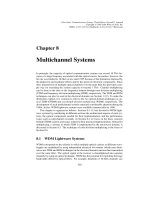
persion, respectively. Chapter 8 focuses on the use of wavelength- and time-division
multiplexing techniques for optical networks. Code-division multiplexing is also a part
of this chapter. The use of optical solitons for fiber-optic systems is discussed in Chapter 9. Coherent lightwave systems are now covered in the last chapter. More than 30%
of the material in Chapter 6–9 is new because of the rapid development of the WDM
technology over the last 5 years. The contents of the book reflect the state of the art of

lightwave transmission systems in 2001.
The primary role of this book is as a graduate-level textbook in the field of optical
communications. An attempt is made to include as much recent material as possible
so that students are exposed to the recent advances in this exciting field. The book can
also serve as a reference text for researchers already engaged in or wishing to enter
the field of optical fiber communications. The reference list at the end of each chapter
is more elaborate than what is common for a typical textbook. The listing of recent
research papers should be useful for researchers using this book as a reference. At
the same time, students can benefit from it if they are assigned problems requiring
reading of the original research papers. A set of problems is included at the end of
each chapter to help both the teacher and the student. Although written primarily for
graduate students, the book can also be used for an undergraduate course at the senior
level with an appropriate selection of topics. Parts of the book can be used for several
other related courses. For example, Chapter 2 can be used for a course on optical
waveguides, and Chapter 3 can be useful for a course on optoelectronics.
Many universities in the United States and elsewhere offer a course on optical communications as a part of their curriculum in electrical engineering, physics, or optics. I
have taught such a course since 1989 to the graduate students of the Institute of Optics,
and this book indeed grew out of my lecture notes. I am aware that it is used as a textbook by many instructors worldwide—a fact that gives me immense satisfaction. I am
acutely aware of a problem that is a side effect of an enlarged revised edition. How can
a teacher fit all this material in a one-semester course on optical communications? I
have to struggle with the same question. In fact, it is impossible to cover the entire book
in one semester. The best solution is to offer a two-semester course covering Chapters
1 through 5 during the first semester, leaving the remainder for the second semester.
However, not many universities may have the luxury of offering a two-semester course
on optical communications. The book can be used for a one-semester course provided
that the instructor makes a selection of topics. For example, Chapter 3 can be skipped
if the students have taken a laser course previously. If only parts of Chapters 6 through
10 are covered to provide students a glimpse of the recent advances, the material can
fit in a single one-semester course offered either at the senior level for undergraduates
or to graduate students.

This edition of the book features a compact disk (CD) on the back cover provided
by the Optiwave Corporation. The CD contains a state-of-the art software package
suitable for designing modern lightwave systems. It also contains additional problems
for each chapter that can be solved by using the software package. Appendix E provides
more details about the software and the problems. It is my hope that the CD will help
to train the students and will prepare them better for an industrial job.
A large number of persons have contributed to this book either directly or indirectly.
It is impossible to mention all of them by name. I thank my graduate students and the


PREFACE

xvii

students who took my course on optical communication systems and helped improve
my class notes through their questions and comments. Thanks are due to many instructors who not only have adopted this book as a textbook for their courses but have also
pointed out the misprints in previous editions, and thus have helped me in improving
the book. I am grateful to my colleagues at the Institute of Optics for numerous discussions and for providing a cordial and productive atmosphere. I appreciated the help
of Karen Rolfe, who typed the first edition of this book and made numerous revisions
with a smile. Last, but not least, I thank my wife, Anne, and my daughters, Sipra,
Caroline, and Claire, for understanding why I needed to spend many weekends on the
book instead of spending time with them.

Govind P. Agrawal
Rochester, NY
December 2001


Fiber-Optic Communications Systems, Third Edition. Govind P. Agrawal
Copyright  2002 John Wiley & Sons, Inc.

ISBNs: 0-471-21571-6 (Hardback); 0-471-22114-7 (Electronic)

Chapter 1

Introduction
A communication system transmits information from one place to another, whether
separated by a few kilometers or by transoceanic distances. Information is often carried by an electromagnetic carrier wave whose frequency can vary from a few megahertz to several hundred terahertz. Optical communication systems use high carrier
frequencies (∼ 100 THz) in the visible or near-infrared region of the electromagnetic
spectrum. They are sometimes called lightwave systems to distinguish them from microwave systems, whose carrier frequency is typically smaller by five orders of magnitude (∼ 1 GHz). Fiber-optic communication systems are lightwave systems that employ optical fibers for information transmission. Such systems have been deployed
worldwide since 1980 and have indeed revolutionized the technology behind telecommunications. Indeed, the lightwave technology, together with microelectronics, is believed to be a major factor in the advent of the “information age.” The objective of
this book is to describe fiber-optic communication systems in a comprehensive manner. The emphasis is on the fundamental aspects, but the engineering issues are also
discussed. The purpose of this introductory chapter is to present the basic concepts and
to provide the background material. Section 1.1 gives a historical perspective on the
development of optical communication systems. In Section 1.2 we cover concepts such
as analog and digital signals, channel multiplexing, and modulation formats. Relative
merits of guided and unguided optical communication systems are discussed in Section 1.3. The last section focuses on the building blocks of a fiber-optic communication
system.

1.1 Historical Perspective
The use of light for communication purposes dates back to antiquity if we interpret
optical communications in a broad sense [1]. Most civilizations have used mirrors, fire
beacons, or smoke signals to convey a single piece of information (such as victory in
a war). Essentially the same idea was used up to the end of the eighteenth century
through signaling lamps, flags, and other semaphore devices. The idea was extended
further, following a suggestion of Claude Chappe in 1792, to transmit mechanically
1


CHAPTER 1. INTRODUCTION

2

Publisher's Note:
Permission to reproduce this image
online was not granted by the
copyright holder. Readers are kindly
asked to refer to the printed version
of this chapter.

Figure 1.1: Schematic illustration of the optical telegraph and its inventor Claude Chappe. (After
Ref. [2]; c 1944 American Association for the Advancement of Science; reprinted with permission.)

coded messages over long distances (∼ 100 km) by the use of intermediate relay stations [2], acting as regenerators or repeaters in the modern-day language. Figure 1.1
shows the basic idea schematically. The first such “optical telegraph” was put in service
between Paris and Lille (two French cities about 200 km apart) in July 1794. By 1830,
the network had expanded throughout Europe [1]. The role of light in such systems
was simply to make the coded signals visible so that they could be intercepted by the
relay stations. The opto-mechanical communication systems of the nineteenth century
were inherently slow. In modern-day terminology, the effective bit rate of such systems
was less than 1 bit per second (B < 1 b/s).

1.1.1 Need for Fiber-Optic Communications
The advent of telegraphy in the 1830s replaced the use of light by electricity and began
the era of electrical communications [3]. The bit rate B could be increased to ∼ 10 b/s
by the use of new coding techniques, such as the Morse code. The use of intermediate
relay stations allowed communication over long distances (∼ 1000 km). Indeed, the
first successful transatlantic telegraph cable went into operation in 1866. Telegraphy
used essentially a digital scheme through two electrical pulses of different durations
(dots and dashes of the Morse code). The invention of the telephone in 1876 brought
a major change inasmuch as electric signals were transmitted in analog form through a

continuously varying electric current [4]. Analog electrical techniques were to dominate communication systems for a century or so.
The development of worldwide telephone networks during the twentieth century
led to many advances in the design of electrical communication systems. The use
of coaxial cables in place of wire pairs increased system capacity considerably. The
first coaxial-cable system, put into service in 1940, was a 3-MHz system capable of
transmitting 300 voice channels or a single television channel. The bandwidth of such
systems is limited by the frequency-dependent cable losses, which increase rapidly for
frequencies beyond 10 MHz. This limitation led to the development of microwave
communication systems in which an electromagnetic carrier wave with frequencies in


1.1. HISTORICAL PERSPECTIVE

3

Figure 1.2: Increase in bit rate–distance product BL during the period 1850–2000. The emergence of a new technology is marked by a solid circle.

the range of 1–10 GHz is used to transmit the signal by using suitable modulation
techniques.
The first microwave system operating at the carrier frequency of 4 GHz was put
into service in 1948. Since then, both coaxial and microwave systems have evolved
considerably and are able to operate at bit rates ∼ 100 Mb/s. The most advanced coaxial system was put into service in 1975 and operated at a bit rate of 274 Mb/s. A severe
drawback of such high-speed coaxial systems is their small repeater spacing (∼ 1 km),
which makes the system relatively expensive to operate. Microwave communication
systems generally allow for a larger repeater spacing, but their bit rate is also limited
by the carrier frequency of such waves. A commonly used figure of merit for communication systems is the bit rate–distance product, BL, where B is the bit rate and L is
the repeater spacing. Figure 1.2 shows how the BL product has increased through technological advances during the last century and a half. Communication systems with
BL ∼ 100 (Mb/s)-km were available by 1970 and were limited to such values because
of fundamental limitations.
It was realized during the second half of the twentieth century that an increase

of several orders of magnitude in the BL product would be possible if optical waves
were used as the carrier. However, neither a coherent optical source nor a suitable
transmission medium was available during the 1950s. The invention of the laser and
its demonstration in 1960 solved the first problem [5]. Attention was then focused
on finding ways for using laser light for optical communications. Many ideas were


CHAPTER 1. INTRODUCTION

4

10000

Bit Rate (Gb/s)

1000
Research
100
10
Commercial
1
0.1
0.01
1980

1985

1990

1995

2000

2005

Year

Figure 1.3: Increase in the capacity of lightwave systems realized after 1980. Commercial
systems (circles) follow research demonstrations (squares) with a few-year lag. The change in
the slope after 1992 is due to the advent of WDM technology.

advanced during the 1960s [6], the most noteworthy being the idea of light confinement
using a sequence of gas lenses [7].
It was suggested in 1966 that optical fibers might be the best choice [8], as they
are capable of guiding the light in a manner similar to the guiding of electrons in copper wires. The main problem was the high losses of optical fibers—fibers available
during the 1960s had losses in excess of 1000 dB/km. A breakthrough occurred in
1970 when fiber losses could be reduced to below 20 dB/km in the wavelength region
near 1 µ m [9]. At about the same time, GaAs semiconductor lasers, operating continuously at room temperature, were demonstrated [10]. The simultaneous availability of
compact optical sources and a low-loss optical fibers led to a worldwide effort for developing fiber-optic communication systems [11]. Figure 1.3 shows the increase in the
capacity of lightwave systems realized after 1980 through several generations of development. As seen there, the commercial deployment of lightwave systems followed the
research and development phase closely. The progress has indeed been rapid as evident from an increase in the bit rate by a factor of 100,000 over a period of less than 25
years. Transmission distances have also increased from 10 to 10,000 km over the same
time period. As a result, the bit rate–distance product of modern lightwave systems can
exceed by a factor of 10 7 compared with the first-generation lightwave systems.

1.1.2 Evolution of Lightwave Systems
The research phase of fiber-optic communication systems started around 1975. The
enormous progress realized over the 25-year period extending from 1975 to 2000 can
be grouped into several distinct generations. Figure 1.4 shows the increase in the BL
product over this time period as quantified through various laboratory experiments [12].

The straight line corresponds to a doubling of the BL product every year. In every


1.1. HISTORICAL PERSPECTIVE

5

Figure 1.4: Increase in the BL product over the period 1975 to 1980 through several generations
of lightwave systems. Different symbols are used for successive generations. (After Ref. [12];
c 2000 IEEE; reprinted with permission.)

generation, BL increases initially but then begins to saturate as the technology matures.
Each new generation brings a fundamental change that helps to improve the system
performance further.
The first generation of lightwave systems operated near 0.8 µ m and used GaAs
semiconductor lasers. After several field trials during the period 1977–79, such systems
became available commercially in 1980 [13]. They operated at a bit rate of 45 Mb/s
and allowed repeater spacings of up to 10 km. The larger repeater spacing compared
with 1-km spacing of coaxial systems was an important motivation for system designers because it decreased the installation and maintenance costs associated with each
repeater.
It was clear during the 1970s that the repeater spacing could be increased considerably by operating the lightwave system in the wavelength region near 1.3 µ m, where
fiber loss is below 1 dB/km. Furthermore, optical fibers exhibit minimum dispersion in
this wavelength region. This realization led to a worldwide effort for the development
of InGaAsP semiconductor lasers and detectors operating near 1.3 µ m. The second
generation of fiber-optic communication systems became available in the early 1980s,
but the bit rate of early systems was limited to below 100 Mb/s because of dispersion in
multimode fibers [14]. This limitation was overcome by the use of single-mode fibers.
A laboratory experiment in 1981 demonstrated transmission at 2 Gb/s over 44 km of
single-mode fiber [15]. The introduction of commercial systems soon followed. By
1987, second-generation lightwave systems, operating at bit rates of up to 1.7 Gb/s

with a repeater spacing of about 50 km, were commercially available.
The repeater spacing of the second-generation lightwave systems was limited by
the fiber losses at the operating wavelength of 1.3 µ m (typically 0.5 dB/km). Losses


6

CHAPTER 1. INTRODUCTION

of silica fibers become minimum near 1.55 µ m. Indeed, a 0.2-dB/km loss was realized in 1979 in this spectral region [16]. However, the introduction of third-generation
lightwave systems operating at 1.55 µ m was considerably delayed by a large fiber
dispersion near 1.55 µ m. Conventional InGaAsP semiconductor lasers could not be
used because of pulse spreading occurring as a result of simultaneous oscillation of
several longitudinal modes. The dispersion problem can be overcome either by using
dispersion-shifted fibers designed to have minimum dispersion near 1.55 µ m or by limiting the laser spectrum to a single longitudinal mode. Both approaches were followed
during the 1980s. By 1985, laboratory experiments indicated the possibility of transmitting information at bit rates of up to 4 Gb/s over distances in excess of 100 km [17].
Third-generation lightwave systems operating at 2.5 Gb/s became available commercially in 1990. Such systems are capable of operating at a bit rate of up to 10 Gb/s [18].
The best performance is achieved using dispersion-shifted fibers in combination with
lasers oscillating in a single longitudinal mode.
A drawback of third-generation 1.55-µ m systems is that the signal is regenerated
periodically by using electronic repeaters spaced apart typically by 60–70 km. The
repeater spacing can be increased by making use of a homodyne or heterodyne detection scheme because its use improves receiver sensitivity. Such systems are referred
to as coherent lightwave systems. Coherent systems were under development worldwide during the 1980s, and their potential benefits were demonstrated in many system
experiments [19]. However, commercial introduction of such systems was postponed
with the advent of fiber amplifiers in 1989.
The fourth generation of lightwave systems makes use of optical amplification for
increasing the repeater spacing and of wavelength-division multiplexing (WDM) for
increasing the bit rate. As evident from different slopes in Fig. 1.3 before and after
1992, the advent of the WDM technique started a revolution that resulted in doubling
of the system capacity every 6 months or so and led to lightwave systems operating at

a bit rate of 10 Tb/s by 2001. In most WDM systems, fiber losses are compensated
periodically using erbium-doped fiber amplifiers spaced 60–80 km apart. Such amplifiers were developed after 1985 and became available commercially by 1990. A 1991
experiment showed the possibility of data transmission over 21,000 km at 2.5 Gb/s,
and over 14,300 km at 5 Gb/s, using a recirculating-loop configuration [20]. This performance indicated that an amplifier-based, all-optical, submarine transmission system
was feasible for intercontinental communication. By 1996, not only transmission over
11,300 km at a bit rate of 5 Gb/s had been demonstrated by using actual submarine
cables [21], but commercial transatlantic and transpacific cable systems also became
available. Since then, a large number of submarine lightwave systems have been deployed worldwide.
Figure 1.5 shows the international network of submarine systems around 2000 [22].
The 27,000-km fiber-optic link around the globe (known as FLAG) became operational
in 1998, linking many Asian and European countries [23]. Another major lightwave
system, known as Africa One was operating by 2000; it circles the African continent
and covers a total transmission distance of about 35,000 km [24]. Several WDM systems were deployed across the Atlantic and Pacific oceans during 1998–2001 in response to the Internet-induced increase in the data traffic; they have increased the total
capacity by orders of magnitudes. A truly global network covering 250,000 km with a


1.1. HISTORICAL PERSPECTIVE

7

Figure 1.5: International undersea network of fiber-optic communication systems around 2000.
(After Ref. [22]; c 2000 Academic; reprinted with permission.)

capacity of 2.56 Tb/s (64 WDM channels at 10 Gb/s over 4 fiber pairs) is scheduled to
be operational in 2002 [25]. Clearly, the fourth-generation systems have revolutionized
the whole field of fiber-optic communications.
The current emphasis of WDM lightwave systems is on increasing the system capacity by transmitting more and more channels through the WDM technique. With
increasing WDM signal bandwidth, it is often not possible to amplify all channels
using a single amplifier. As a result, new kinds of amplification schemes are being
explored for covering the spectral region extending from 1.45 to 1.62 µ m. This approach led in 2000 to a 3.28-Tb/s experiment in which 82 channels, each operating at

40 Gb/s, were transmitted over 3000 km, resulting in a BL product of almost 10,000
(Tb/s)-km. Within a year, the system capacity could be increased to nearly 11 Tb/s
(273 WDM channels, each operating at 40 Gb/s) but the transmission distance was
limited to 117 km [26]. In another record experiment, 300 channels, each operating
at 11.6 Gb/s, were transmitted over 7380 km, resulting in a BL product of more than
25,000 (Tb/s)-km [27]. Commercial terrestrial systems with the capacity of 1.6 Tb/s
were available by the end of 2000, and the plans were underway to extend the capacity
toward 6.4 Tb/s. Given that the first-generation systems had a capacity of 45 Mb/s in
1980, it is remarkable that the capacity has jumped by a factor of more than 10,000
over a period of 20 years.
The fifth generation of fiber-optic communication systems is concerned with extending the wavelength range over which a WDM system can operate simultaneously.
The conventional wavelength window, known as the C band, covers the wavelength
range 1.53–1.57 µ m. It is being extended on both the long- and short-wavelength sides,
resulting in the L and S bands, respectively. The Raman amplification technique can be
used for signals in all three wavelength bands. Moreover, a new kind of fiber, known
as the dry fiber has been developed with the property that fiber losses are small over
the entire wavelength region extending from 1.30 to 1.65 µ m [28]. Availability of such
fibers and new amplification schemes may lead to lightwave systems with thousands of
WDM channels.
The fifth-generation systems also attempt to increase the bit rate of each channel


8

CHAPTER 1. INTRODUCTION

within the WDM signal. Starting in 2000, many experiments used channels operating at
40 Gb/s; migration toward 160 Gb/s is also likely in the future. Such systems require an
extremely careful management of fiber dispersion. An interesting approach is based on
the concept of optical solitons—pulses that preserve their shape during propagation in

a lossless fiber by counteracting the effect of dispersion through the fiber nonlinearity.
Although the basic idea was proposed [29] as early as 1973, it was only in 1988 that
a laboratory experiment demonstrated the feasibility of data transmission over 4000
km by compensating the fiber loss through Raman amplification [30]. Erbium-doped
fiber amplifiers were used for soliton amplification starting in 1989. Since then, many
system experiments have demonstrated the eventual potential of soliton communication
systems. By 1994, solitons were transmitted over 35,000 km at 10 Gb/s and over
24,000 km at 15 Gb/s [31]. Starting in 1996, the WDM technique was also used for
solitons in combination with dispersion management. In a 2000 experiment, up to 27
WDM channels, each operating at 20 Gb/s, were transmitted over 9000 km using a
hybrid amplification scheme [32].
Even though the fiber-optic communication technology is barely 25 years old, it has
progressed rapidly and has reached a certain stage of maturity. This is also apparent
from the publication of a large number of books on optical communications and WDM
networks since 1995 [33]–[55]. This third edition of a book, first published in 1992, is
intended to present an up-to-date account of fiber-optic communications systems with
emphasis on recent developments.

1.2 Basic Concepts
This section introduces a few basic concepts common to all communication systems.
We begin with a description of analog and digital signals and describe how an analog signal can be converted into digital form. We then consider time- and frequencydivision multiplexing of input signals, and conclude with a discussion of various modulation formats.

1.2.1 Analog and Digital Signals
In any communication system, information to be transmitted is generally available as
an electrical signal that may take analog or digital form [56]. In the analog case, the
signal (e. g., electric current) varies continuously with time, as shown schematically in
Fig. 1.6(a). Familiar examples include audio and video signals resulting when a microphone converts voice or a video camera converts an image into an electrical signal.
By contrast, the digital signal takes only a few discrete values. In the binary representation of a digital signal only two values are possible. The simplest case of a binary
digital signal is one in which the electric current is either on or off, as shown in Fig.
1.6(b). These two possibilities are called “bit 1” and “bit 0” (bit is a contracted form of

binary digit). Each bit lasts for a certain period of time T B , known as the bit period or
bit slot. Since one bit of information is conveyed in a time interval T B , the bit rate B,
defined as the number of bits per second, is simply B = T B−1 . A well-known example of
digital signals is provided by computer data. Each letter of the alphabet together with


1.2. BASIC CONCEPTS

9

Figure 1.6: Representation of (a) an analog signal and (b) a digital signal.

other common symbols (decimal numerals, punctuation marks, etc.) is assigned a code
number (ASCII code) in the range 0–127 whose binary representation corresponds to
a 7-bit digital signal. The original ASCII code has been extended to represent 256
characters transmitted through 8-bit bytes. Both analog and digital signals are characterized by their bandwidth, which is a measure of the spectral contents of the signal.
The signal bandwidth represents the range of frequencies contained within the signal
and is determined mathematically through its Fourier transform.
An analog signal can be converted into digital form by sampling it at regular intervals of time [56]. Figure 1.7 shows the conversion method schematically. The sampling
rate is determined by the bandwidth ∆ f of the analog signal. According to the sampling theorem [57]–[59], a bandwidth-limited signal can be fully represented by discrete samples, without any loss of information, provided that the sampling frequency
fs satisfies the Nyquist criterion [60], f s ≥ 2∆ f . The first step consists of sampling
the analog signal at the right frequency. The sampled values can take any value in the
range 0 ≤ A ≤ A max , where Amax is the maximum amplitude of the given analog signal.
Let us assume that Amax is divided into M discrete (not necessarily equally spaced) intervals. Each sampled value is quantized to correspond to one of these discrete values.
Clearly, this procedure leads to additional noise, known as quantization noise, which
adds to the noise already present in the analog signal.
The effect of quantization noise can be minimized by choosing the number of discrete levels such that M > Amax /AN , where AN is the root-mean-square noise amplitude
of the analog signal. The ratio A max /AN is called the dynamic range and is related to

CHAPTER 1. INTRODUCTION

10

Figure 1.7: Three steps of (a) sampling, (b) quantization, and (c) coding required for converting
an analog signal into a binary digital signal.

the signal-to-noise ratio (SNR) by the relation
SNR = 20 log10 (Amax /AN ),

(1.2.1)

where SNR is expressed in decibel (dB) units. Any ratio R can be converted into
decibels by using the general definition 10 log 10 R (see Appendix A). Equation (1.2.1)
contains a factor of 20 in place of 10 simply because the SNR for electrical signals is
defined with respect to the electrical power, whereas A is related to the electric current
(or voltage).
The quantized sampled values can be converted into digital format by using a suitable conversion technique. In one scheme, known as pulse-position modulation, pulse
position within the bit slot is a measure of the sampled value. In another, known as
pulse-duration modulation, the pulse width is varied from bit to bit in accordance with
the sampled value. These techniques are rarely used in practical optical communication
systems, since it is difficult to maintain the pulse position or pulse width to high accuracy during propagation inside the fiber. The technique used almost universally, known
as pulse-code modulation (PCM), is based on a binary scheme in which information
is conveyed by the absence or the presence of pulses that are otherwise identical. A
binary code is used to convert each sampled value into a string of 1 and 0 bits. The