Tài liệu Fibre optic communication systems P2 pdf
Bạn đang xem bản rút gọn của tài liệu. Xem và tải ngay bản đầy đủ của tài liệu tại đây (501 KB, 54 trang )
Chapter 2
Optical Fibers
The phenomenon of total internal reflection, responsible for guiding of light in opti-
cal fibers, has been known since 1854 [1]. Although glass fibers were made in the
1920s [2]–[4], their use became practical only in the 1950s, when the use of a cladding
layer led to considerable improvement in their guiding characteristics [5]–[7]. Before
1970, optical fibers were used mainly for medical imaging over short distances [8].
Their use for communication purposes was considered impractical because of high
losses (∼ 1000 dB/km). However, the situation changed drastically in 1970 when, fol-
lowing an earlier suggestion [9], the loss of optical fibers was reduced to below 20
dB/km [10]. Further progress resulted by 1979 in a loss of only 0.2 dB/km near the
1.55-
µ
m spectral region [11]. The availability of low-loss fibers led to a revolution
in the field of lightwave technology and started the era of fiber-optic communications.
Several books devoted entirely to optical fibers cover numerous advances made in their
design and understanding [12]–[21]. This chapter focuses on the role of optical fibers
as a communication channel in lightwave systems. In Section 2.1 we use geometrical-
optics description to explain the guiding mechanism and introduce the related basic
concepts. Maxwell’s equations are used in Section 2.2 to describe wave propagation
in optical fibers. The origin of fiber dispersion is discussed in Section 2.3, and Section
2.4 considers limitations on the bit rate and the transmission distance imposed by fiber
dispersion. The loss mechanisms in optical fibers are discussed in Section 2.5, and
Section 2.6 is devoted to a discussion of the nonlinear effects. The last section covers
manufacturing details and includes a discussion of the design of fiber cables.
2.1 Geometrical-Optics Description
In its simplest form an optical fiber consists of a cylindrical core of silica glass sur-
rounded by a cladding whose refractive index is lower than that of the core. Because of
an abrupt index change at the core–cladding interface, such fibers are called step-index
fibers. In a different type of fiber, known as graded-index fiber, the refractive index
decreases gradually inside the core. Figure 2.1 shows schematically the index profile
and the cross section for the two kinds of fibers. Considerable insight in the guiding
23
Fiber-Optic Communications Systems, Third Edition. Govind P. Agrawal
Copyright
2002 John Wiley & Sons, Inc.
ISBNs: 0-471-21571-6 (Hardback); 0-471-22114-7 (Electronic)
24
CHAPTER 2. OPTICAL FIBERS
Figure 2.1: Cross section and refractive-index profile for step-index and graded-index fibers.
properties of optical fibers can be gained by using a ray picture based on geometrical
optics [22]. The geometrical-optics description, although approximate, is valid when
the core radius a is much larger than the light wavelength
λ
. When the two become
comparable, it is necessary to use the wave-propagation theory of Section 2.2.
2.1.1 Step-Index Fibers
Consider the geometry of Fig. 2.2, where a ray making an angle
θ
i
with the fiber axis
is incident at the core center. Because of refraction at the fiber–air interface, the ray
bends toward the normal. The angle
θ
r
of the refracted ray is given by [22]
n
0
sin
θ
i
= n
1
sin
θ
r
, (2.1.1)
where n
1
and n
0
are the refractive indices of the fiber core and air, respectively. The re-
fracted ray hits the core–cladding interface and is refracted again. However, refraction
is possible only for an angle of incidence
φ
such that sin
φ
< n
2
/n
1
. For angles larger
than a critical angle
φ
c
, defined by [22]
sin
φ
c
= n
2
/n
1
, (2.1.2)
where n
2
is the cladding index, the ray experiences total internal reflection at the core–
cladding interface. Since such reflections occur throughout the fiber length, all rays
with
φ
>
φ
c
remain confined to the fiber core. This is the basic mechanism behind light
confinement in optical fibers.
2.1. GEOMETRICAL-OPTICS DESCRIPTION
25
Figure 2.2: Light confinement through total internal reflection in step-index fibers. Rays for
which
φ
<
φ
c
are refracted out of the core.
One can use Eqs. (2.1.1) and (2.1.2) to find the maximum angle that the incident
ray should make with the fiber axis to remain confined inside the core. Noting that
θ
r
=
π
/2−
φ
c
for such a ray and substituting it in Eq. (2.1.1), we obtain
n
0
sin
θ
i
= n
1
cos
φ
c
=(n
2
1
− n
2
2
)
1/2
. (2.1.3)
In analogy with lenses, n
0
sin
θ
i
is known as the numerical aperture (NA) of the fiber.
It represents the light-gathering capacity of an optical fiber. For n
1
n
2
the NA can be
approximated by
NA = n
1
(2∆)
1/2
, ∆ =(n
1
− n
2
)/n
1
, (2.1.4)
where ∆ is the fractional index change at the core–cladding interface. Clearly, ∆ should
be made as large as possible in order to couple maximum light into the fiber. How-
ever, such fibers are not useful for the purpose of optical communications because of a
phenomenon known as multipath dispersion or modal dispersion (the concept of fiber
modes is introduced in Section 2.2).
Multipath dispersion can be understood by referring to Fig. 2.2, where different
rays travel along paths of different lengths. As a result, these rays disperse in time at
the output end of the fiber even if they were coincident at the input end and traveled
at the same speed inside the fiber. A short pulse (called an impulse) would broaden
considerably as a result of different path lengths. One can estimate the extent of pulse
broadening simply by considering the shortest and longest ray paths. The shortest path
occurs for
θ
i
= 0 and is just equal to the fiber length L. The longest path occurs for
θ
i
given by Eq. (2.1.3) and has a length L/sin
φ
c
. By taking the velocity of propagation
v = c/n
1
, the time delay is given by
∆T =
n
1
c
L
sin
φ
c
− L
=
L
c
n
2
1
n
2
∆. (2.1.5)
The time delay between the two rays taking the shortest and longest paths is a measure
of broadening experienced by an impulse launched at the fiber input.
We can relate ∆T to the information-carrying capacity of the fiber measured through
the bit rate B. Although a precise relation between B and ∆T depends on many details,
26
CHAPTER 2. OPTICAL FIBERS
such as the pulse shape, it is clear intuitively that ∆T should be less than the allocated
bit slot (T
B
= 1/B). Thus, an order-of-magnitude estimate of the bit rate is obtained
from the condition B∆T < 1. By using Eq. (2.1.5) we obtain
BL <
n
2
n
2
1
c
∆
. (2.1.6)
This condition provides a rough estimate of a fundamental limitation of step-index
fibers. As an illustration, consider an unclad glass fiber with n
1
= 1.5 and n
2
= 1.
The bit rate–distance product of such a fiber is limited to quite small values since
BL < 0.4 (Mb/s)-km. Considerable improvement occurs for cladded fibers with a small
index step. Most fibers for communication applications are designed with ∆ < 0.01.
As an example, BL < 100 (Mb/s)-km for ∆ = 2× 10
−3
. Such fibers can communicate
data at a bit rate of 10 Mb/s over distances up to 10 km and may be suitable for some
local-area networks.
Two remarks are in order concerning the validity of Eq. (2.1.6). First, it is obtained
by considering only rays that pass through the fiber axis after each total internal re-
flection. Such rays are called meridional rays. In general, the fiber also supports skew
rays, which travel at angles oblique to the fiber axis. Skew rays scatter out of the core at
bends and irregularities and are not expected to contribute significantly to Eq. (2.1.6).
Second, even the oblique meridional rays suffer higher losses than paraxial meridional
rays because of scattering. Equation (2.1.6) provides a conservative estimate since all
rays are treated equally. The effect of intermodal dispersion can be considerably re-
duced by using graded-index fibers, which are discussed in the next subsection. It can
be eliminated entirely by using the single-mode fibers discussed in Section 2.2.
2.1.2 Graded-Index Fibers
The refractive index of the core in graded-index fibers is not constant but decreases
gradually from its maximum value n
1
at the core center to its minimum value n
2
at
the core–cladding interface. Most graded-index fibers are designed to have a nearly
quadratic decrease and are analyzed by using
α
-profile, given by
n(
ρ
)=
n
1
[1− ∆(
ρ
/a)
α
];
ρ
< a,
n
1
(1− ∆)=n
2
;
ρ
≥ a,
(2.1.7)
where a is the core radius. The parameter
α
determines the index profile. A step-index
profile is approached in the limit of large
α
.Aparabolic-index fiber corresponds to
α
= 2.
It is easy to understand qualitatively why intermodal or multipath dispersion is re-
duced for graded-index fibers. Figure 2.3 shows schematically paths for three different
rays. Similar to the case of step-index fibers, the path is longer for more oblique rays.
However, the ray velocity changes along the path because of variations in the refractive
index. More specifically, the ray propagating along the fiber axis takes the shortest path
but travels most slowly as the index is largest along this path. Oblique rays have a large
part of their path in a medium of lower refractive index, where they travel faster. It is
therefore possible for all rays to arrive together at the fiber output by a suitable choice
of the refractive-index profile.
2.1. GEOMETRICAL-OPTICS DESCRIPTION
27
Figure 2.3: Ray trajectories in a graded-index fiber.
Geometrical optics can be used to show that a parabolic-index profile leads to
nondispersive pulse propagation within the paraxial approximation. The trajectory
of a paraxial ray is obtained by solving [22]
d
2
ρ
dz
2
=
1
n
dn
d
ρ
, (2.1.8)
where
ρ
is the radial distance of the ray from the axis. By using Eq. (2.1.7) for
ρ
<
a with
α
= 2, Eq. (2.1.8) reduces to an equation of harmonic oscillator and has the
general solution
ρ
=
ρ
0
cos(pz)+(
ρ
0
/p) sin(pz), (2.1.9)
where p =(2∆/a
2
)
1/2
and
ρ
0
and
ρ
0
are the position and the direction of the input
ray, respectively. Equation (2.1.9) shows that all rays recover their initial positions
and directions at distances z = 2m
π
/p, where m is an integer (see Fig. 2.3). Such a
complete restoration of the input implies that a parabolic-index fiber does not exhibit
intermodal dispersion.
The conclusion above holds only within the paraxial and the geometrical-optics ap-
proximations, both of which must be relaxed for practical fibers. Intermodal dispersion
in graded-index fibers has been studied extensively by using wave-propagation tech-
niques [13]–[15]. The quantity ∆T /L, where ∆T is the maximum multipath delay in
a fiber of length L, is found to vary considerably with
α
. Figure 2.4 shows this varia-
tion for n
1
= 1.5 and ∆ = 0.01. The minimum dispersion occurs for
α
= 2(1− ∆) and
depends on ∆ as [23]
∆T /L = n
1
∆
2
/8c. (2.1.10)
The limiting bit rate–distance product is obtained by using the criterion ∆T < 1/B and
is given by
BL < 8c/n
1
∆
2
. (2.1.11)
The right scale in Fig. 2.4 shows the BL product as a function of
α
. Graded-index fibers
with a suitably optimized index profile can communicate data at a bit rate of 100 Mb/s
over distances up to 100 km. The BL product of such fibers is improved by nearly
three orders of magnitude over that of step-index fibers. Indeed, the first generation
28
CHAPTER 2. OPTICAL FIBERS
Figure 2.4: Variation of intermodal dispersion ∆T/L with the profile parameter
α
for a graded-
index fiber. The scale on the right shows the corresponding bit rate–distance product.
of lightwave systems used graded-index fibers. Further improvement is possible only
by using single-mode fibers whose core radius is comparable to the light wavelength.
Geometrical optics cannot be used for such fibers.
Although graded-index fibers are rarely used for long-haul links, the use of graded-
index plastic optical fibers for data-link applications has attracted considerable atten-
tion during the 1990s [24]–[29]. Such fibers have a relatively large core, resulting in
a high numerical aperture and high coupling efficiency but they exhibit high losses
(typically exceeding 50 dB/km). The BL product of plastic fibers, however, exceeds
2 (Gb/s)-km because of a graded-index profile [24]. As a result, they can be used to
transmit data at bit rates > 1 Gb/s over short distances of 1 km or less. In a 1996
demonstration, a 10-Gb/s signal was transmitted over 0.5 km with a bit-error rate of
less than 10
−11
[26]. Graded-index plastic optical fibers provide an ideal solution for
transferring data among computers and are becoming increasingly important for Eth-
ernet applications requiring bit rates in excess of 1 Gb/s.
2.2 Wave Propagation
In this section we consider propagation of light in step-index fibers by using Maxwell’s
equations for electromagnetic waves. These equations are introduced in Section 2.2.1.
The concept of fiber modes is discussed in Section 2.2.2, where the fiber is shown to
support a finite number of guided modes. Section 2.2.3 focuses on how a step-index
fiber can be designed to support only a single mode and discusses the properties of
single-mode fibers.
2.2. WAVE PROPAGATION
29
2.2.1 Maxwell’s Equations
Like all electromagnetic phenomena, propagation of optical fields in fibers is governed
by Maxwell’s equations. For a nonconducting medium without free charges, these
equations take the form [30] (in SI units; see Appendix A)
∇× E = −
∂
B/
∂
t, (2.2.1)
∇× H =
∂
D/
∂
t, (2.2.2)
∇· D = 0, (2.2.3)
∇· B = 0, (2.2.4)
where E and H are the electric and magnetic field vectors, respectively, and D and B
are the corresponding flux densities. The flux densities are related to the field vectors
by the constitutive relations [30]
D =
ε
0
E + P, (2.2.5)
B =
µ
0
H + M, (2.2.6)
where
ε
0
is the vacuum permittivity,
µ
0
is the vacuum permeability, and P and M are
the induced electric and magnetic polarizations, respectively. For optical fibers M = 0
because of the nonmagnetic nature of silica glass.
Evaluation of the electric polarization P requires a microscopic quantum-mechanical
approach. Although such an approach is essential when the optical frequency is near
a medium resonance, a phenomenological relation between P and E can be used far
from medium resonances. This is the case for optical fibers in the wavelength region
0.5–2
µ
m, a range that covers the low-loss region of optical fibers that is of interest
for fiber-optic communication systems. In general, the relation between P and E can
be nonlinear. Although the nonlinear effects in optical fibers are of considerable in-
terest [31] and are covered in Section 2.6, they can be ignored in a discussion of fiber
modes. P is then related to E by the relation
P(r,t)=
ε
0
∞
−∞
χ
(r,t − t
)E(r,t
)dt
. (2.2.7)
Linear susceptibility
χ
is, in general, a second-rank tensor but reduces to a scalar for
an isotropic medium such as silica glass. Optical fibers become slightly birefringent
because of unintentional variations in the core shape or in local strain; such birefrin-
gent effects are considered in Section 2.2.3. Equation (2.2.7) assumes a spatially local
response. However, it includes the delayed nature of the temporal response, a feature
that has important implications for optical fiber communications through chromatic
dispersion.
Equations (2.2.1)–(2.2.7) provide a general formalism for studying wave propaga-
tion in optical fibers. In practice, it is convenient to use a single field variable E.By
taking the curl of Eq. (2.2.1) and using Eqs. (2.2.2), (2.2.5), and (2.2.6), we obtain the
wave equation
∇× ∇× E = −
1
c
2
∂
2
E
∂
t
2
−
µ
0
∂
2
P
∂
t
2
, (2.2.8)
30
CHAPTER 2. OPTICAL FIBERS
where the speed of light in vacuum is defined as usual by c =(
µ
0
ε
0
)
−1/2
. By introduc-
ing the Fourier transform of E(r,t) through the relation
˜
E(r,
ω
)=
∞
−∞
E(r,t) exp(i
ω
t) dt, (2.2.9)
as well as a similar relation for P(r,t), and by using Eq. (2.2.7), Eq. (2.2.8) can be
written in the frequency domain as
∇× ∇×
˜
E = −
ε
(r,
ω
)(
ω
2
/c
2
)
˜
E, (2.2.10)
where the frequency-dependent dielectric constant is defined as
ε
(r,
ω
)=1 +
˜
χ
(r,
ω
), (2.2.11)
and
˜
χ
(r,
ω
) is the Fourier transform of
χ
(r,t). In general,
ε
(r,
ω
) is complex. Its real
and imaginary parts are related to the refractive index n and the absorption coefficient
α
by the definition
ε
=(n + i
α
c/2
ω
)
2
. (2.2.12)
By using Eqs. (2.2.11) and (2.2.12), n and
α
are related to
˜
χ
as
n =(1 + Re
˜
χ
)
1/2
, (2.2.13)
α
=(
ω
/nc)Im
˜
χ
, (2.2.14)
where Re and Im stand for the real and imaginary parts, respectively. Both n and
α
are frequency dependent. The frequency dependence of n is referred to as chromatic
dispersion or simply as material dispersion. In Section 2.3, fiber dispersion is shown
to limit the performance of fiber-optic communication systems in a fundamental way.
Two further simplifications can be made before solving Eq. (2.2.10). First,
ε
can
be taken to be real and replaced by n
2
because of low optical losses in silica fibers.
Second, since n(r,
ω
) is independent of the spatial coordinate r in both the core and the
cladding of a step-index fiber, one can use the identity
∇× ∇×
˜
E≡ ∇(∇·
˜
E)− ∇
2
˜
E = −∇
2
˜
E, (2.2.15)
where we used Eq. (2.2.3) and the relation
˜
D =
ε
˜
E to set ∇·
˜
E = 0. This simplification
is made even for graded-index fibers. Equation (2.2.15) then holds approximately as
long as the index changes occur over a length scale much longer than the wavelength.
By using Eq. (2.2.15) in Eq. (2.2.10), we obtain
∇
2
˜
E + n
2
(
ω
)k
2
0
˜
E = 0, (2.2.16)
where the free-space wave number k
0
is defined as
k
0
=
ω
/c = 2
π
/
λ
, (2.2.17)
and
λ
is the vacuum wavelength of the optical field oscillating at the frequency
ω
.
Equation (2.2.16) is solved next to obtain the optical modes of step-index fibers.
2.2. WAVE PROPAGATION
31
2.2.2 Fiber Modes
The concept of the mode is a general concept in optics occurring also, for example, in
the theory of lasers. An optical mode refers to a specific solution of the wave equation
(2.2.16) that satisfies the appropriate boundary conditions and has the property that its
spatial distribution does not change with propagation. The fiber modes can be classified
as guided modes, leaky modes, and radiation modes [14]. As one might expect, sig-
nal transmission in fiber-optic communication systems takes place through the guided
modes only. The following discussion focuses exclusively on the guided modes of a
step-index fiber.
To take advantage of the cylindrical symmetry, Eq. (2.2.16) is written in the cylin-
drical coordinates
ρ
,
φ
, and z as
∂
2
E
z
∂ρ
2
+
1
ρ
∂
E
z
∂ρ
+
1
ρ
2
∂
2
E
z
∂φ
2
+
∂
2
E
z
∂
z
2
+ n
2
k
2
0
E
z
= 0, (2.2.18)
where for a step-index fiber of core radius a, the refractive index n is of the form
n =
n
1
;
ρ
≤ a,
n
2
;
ρ
> a.
(2.2.19)
For simplicity of notation, the tilde over
˜
E has been dropped and the frequency de-
pendence of all variables is implicitly understood. Equation (2.2.18) is written for the
axial component E
z
of the electric field vector. Similar equations can be written for the
other five components of E and H. However, it is not necessary to solve all six equa-
tions since only two components out of six are independent. It is customary to choose
E
z
and H
z
as the independent components and obtain E
ρ
, E
φ
, H
ρ
, and H
φ
in terms of
them. Equation (2.2.18) is easily solved by using the method of separation of variables
and writing E
z
as
E
z
(
ρ
,
φ
,z)=F(
ρ
)Φ(
φ
)Z(z). (2.2.20)
By using Eq. (2.2.20) in Eq. (2.2.18), we obtain the three ordinary differential equa-
tions:
d
2
Z/dz
2
+
β
2
Z = 0, (2.2.21)
d
2
Φ/d
φ
2
+ m
2
Φ = 0, (2.2.22)
d
2
F
d
ρ
2
+
1
ρ
dF
d
ρ
+
n
2
k
2
0
−
β
2
−
m
2
ρ
2
F = 0. (2.2.23)
Equation (2.2.21) has a solution of the form Z = exp(i
β
z), where
β
has the physical
significance of the propagation constant. Similarly, Eq. (2.2.22) has a solution Φ =
exp(im
φ
), but the constant m is restricted to take only integer values since the field
must be periodic in
φ
with a period of 2
π
.
Equation (2.2.23) is the well-known differential equation satisfied by the Bessel
functions [32]. Its general solution in the core and cladding regions can be written as
F(
ρ
)=
AJ
m
(p
ρ
)+A
Y
m
(p
ρ
);
ρ
≤ a,
CK
m
(q
ρ
)+C
I
m
(q
ρ
);
ρ
> a,
(2.2.24)
32
CHAPTER 2. OPTICAL FIBERS
where A, A
, C, and C
are constants and J
m
, Y
m
, K
m
, and I
m
are different kinds of Bessel
functions [32]. The parameters p and q are defined by
p
2
= n
2
1
k
2
0
−
β
2
, (2.2.25)
q
2
=
β
2
− n
2
2
k
2
0
. (2.2.26)
Considerable simplification occurs when we use the boundary condition that the optical
field for a guided mode should be finite at
ρ
= 0 and decay to zero at
ρ
= ∞. Since
Y
m
(p
ρ
) has a singularity at
ρ
= 0, F(0) can remain finite only if A
= 0. Similarly
F(
ρ
) vanishes at infinity only if C
= 0. The general solution of Eq. (2.2.18) is thus of
the form
E
z
=
AJ
m
(p
ρ
)exp(im
φ
)exp(i
β
z) ;
ρ
≤ a,
CK
m
(q
ρ
)exp(im
φ
)exp(i
β
z);
ρ
> a.
(2.2.27)
The same method can be used to obtain H
z
which also satisfies Eq. (2.2.18). Indeed,
the solution is the same but with different constants B and D, that is,
H
z
=
BJ
m
(p
ρ
)exp(im
φ
)exp(i
β
z) ;
ρ
≤ a,
DK
m
(q
ρ
)exp(im
φ
)exp(i
β
z);
ρ
> a.
(2.2.28)
The other four components E
ρ
, E
φ
, H
ρ
, and H
φ
can be expressed in terms of E
z
and H
z
by using Maxwell’s equations. In the core region, we obtain
E
ρ
=
i
p
2
β
∂
E
z
∂ρ
+
µ
0
ω
ρ
∂
H
z
∂φ
, (2.2.29)
E
φ
=
i
p
2
β
ρ
∂
E
z
∂φ
−
µ
0
ω
∂
H
z
∂ρ
, (2.2.30)
H
ρ
=
i
p
2
β
∂
H
z
∂ρ
−
ε
0
n
2
ω
ρ
∂
E
z
∂φ
, (2.2.31)
H
φ
=
i
p
2
β
ρ
∂
H
z
∂φ
+
ε
0
n
2
ω
∂
E
z
∂ρ
. (2.2.32)
These equations can be used in the cladding region after replacing p
2
by −q
2
.
Equations (2.2.27)–(2.2.32) express the electromagnetic field in the core and clad-
ding regions of an optical fiber in terms of four constants A, B, C, and D. These
constants are determined by applying the boundary condition that the tangential com-
ponents of E and H be continuous across the core–cladding interface. By requiring
the continuity of E
z
, H
z
, E
φ
, and H
φ
at
ρ
= a, we obtain a set of four homogeneous
equations satisfied by A, B, C, and D [19]. These equations have a nontrivial solution
only if the determinant of the coefficient matrix vanishes. After considerable algebraic
details, this condition leads us to the following eigenvalue equation [19]–[21]:
J
m
(pa)
pJ
m
(pa)
+
K
m
(qa)
qK
m
(qa)
J
m
(pa)
pJ
m
(pa)
+
n
2
2
n
2
1
K
m
(qa)
qK
m
(qa)
=
m
2
a
2
1
p
2
+
1
q
2
1
p
2
+
n
2
2
n
2
1
1
q
2
, (2.2.33)
2.2. WAVE PROPAGATION
33
where a prime indicates differentiation with respect to the argument.
For a given set of the parameters k
0
, a, n
1
, and n
2
, the eigenvalue equation (2.2.33)
can be solved numerically to determine the propagation constant
β
. In general, it
may have multiple solutions for each integer value of m. It is customary to enumerate
these solutions in descending numerical order and denote them by
β
mn
for a given m
(n = 1,2,....). Each value
β
mn
corresponds to one possible mode of propagation of the
optical field whose spatial distribution is obtained from Eqs. (2.2.27)–(2.2.32). Since
the field distribution does not change with propagation except for a phase factor and sat-
isfies all boundary conditions, it is an optical mode of the fiber. In general, both E
z
and
H
z
are nonzero (except for m = 0), in contrast with the planar waveguides, for which
one of them can be taken to be zero. Fiber modes are therefore referred to as hybrid
modes and are denoted by HE
mn
or EH
mn
, depending on whether H
z
or E
z
dominates.
In the special case m = 0, HE
0n
and EH
0n
are also denoted by TE
0n
and TM
0n
, respec-
tively, since they correspond to transverse-electric (E
z
= 0) and transverse-magnetic
(H
z
= 0) modes of propagation. A different notation LP
mn
is sometimes used for
weakly guiding fibers [33] for which both E
z
and H
z
are nearly zero (LP stands for
linearly polarized modes).
A mode is uniquely determined by its propagation constant
β
. It is useful to in-
troduce a quantity ¯n =
β
/k
0
, called the mode index or effective index and having the
physical significance that each fiber mode propagates with an effective refractive in-
dex ¯n whose value lies in the range n
1
> ¯n > n
2
. A mode ceases to be guided when
¯n≤ n
2
. This can be understood by noting that the optical field of guided modes decays
exponentially inside the cladding layer since [32]
K
m
(q
ρ
)=(
π
/2q
ρ
)
1/2
exp(−q
ρ
) for q
ρ
1. (2.2.34)
When ¯n ≤ n
2
, q
2
≤ 0 from Eq. (2.2.26) and the exponential decay does not occur. The
mode is said to reach cutoff when q becomes zero or when ¯n = n
2
. From Eq. (2.2.25),
p = k
0
(n
2
1
−n
2
2
)
1/2
when q = 0. A parameter that plays an important role in determining
the cutoff condition is defined as
V = k
0
a(n
2
1
− n
2
2
)
1/2
≈ (2
π
/
λ
)an
1
√
2∆. (2.2.35)
It is called the normalized frequency (V ∝
ω
) or simply the V parameter. It is also
useful to introduce a normalized propagation constant b as
b =
β
/k
0
− n
2
n
1
− n
2
=
¯n− n
2
n
1
− n
2
. (2.2.36)
Figure 2.5 shows a plot of b as a function of V for a few low-order fiber modes obtained
by solving the eigenvalue equation (2.2.33). A fiber with a large value of V supports
many modes. A rough estimate of the number of modes for such a multimode fiber
is given by V
2
/2 [23]. For example, a typical multimode fiber with a = 25
µ
m and
∆ = 5×10
−3
has V 18 at
λ
= 1.3
µ
m and would support about 162 modes. However,
the number of modes decreases rapidly as V is reduced. As seen in Fig. 2.5, a fiber with
V = 5 supports seven modes. Below a certain value of V all modes except the HE
11
mode reach cutoff. Such fibers support a single mode and are called single-mode fibers.
The properties of single-mode fibers are described next.
34
CHAPTER 2. OPTICAL FIBERS
Figure 2.5: Normalized propagation constant b as a function of normalized frequency V for a
few low-order fiber modes. The right scale shows the mode index ¯n. (After Ref. [34];
c
1981
Academic Press; reprinted with permission.)
2.2.3 Single-Mode Fibers
Single-mode fibers support only the HE
11
mode, also known as the fundamental mode
of the fiber. The fiber is designed such that all higher-order modes are cut off at the
operating wavelength. As seen in Fig. 2.5, the V parameter determines the number of
modes supported by a fiber. The cutoff condition of various modes is also determined
by V . The fundamental mode has no cutoff and is always supported by a fiber.
Single-Mode Condition
The single-mode condition is determined by the value of V at which the TE
01
and TM
01
modes reach cutoff (see Fig. 2.5). The eigenvalue equations for these two modes can
be obtained by setting m = 0 in Eq. (2.2.33) and are given by
pJ
0
(pa)K
0
(qa)+qJ
0
(pa)K
0
(qa)=0, (2.2.37)
pn
2
2
J
0
(pa)K
0
(qa)+qn
2
1
J
0
(pa)K
0
(qa)=0. (2.2.38)
A mode reaches cutoff when q = 0. Since pa = V when q = 0, the cutoff condition for
both modes is simply given by J
0
(V)=0. The smallest value of V for which J
0
(V)=0
is 2.405. A fiber designed such that V < 2.405 supports only the fundamental HE
11
mode. This is the single-mode condition.
2.2. WAVE PROPAGATION
35
We can use Eq. (2.2.35) to estimate the core radius of single-mode fibers used
in lightwave systems. For the operating wavelength range 1.3–1.6
µ
m, the fiber is
generally designed to become single mode for
λ
> 1.2
µ
m. By taking
λ
= 1.2
µ
m,
n
1
= 1.45, and ∆ = 5× 10
−3
, Eq. (2.2.35) shows that V < 2.405 for a core radius
a < 3.2
µ
m. The required core radius can be increased to about 4
µ
m by decreasing ∆
to 3× 10
−3
. Indeed, most telecommunication fibers are designed with a ≈ 4
µ
m.
The mode index ¯n at the operating wavelength can be obtained by using Eq. (2.2.36),
according to which
¯n = n
2
+ b(n
1
− n
2
)≈ n
2
(1 + b∆) (2.2.39)
and by using Fig. 2.5, which provides b as a function of V for the HE
11
mode. An
analytic approximation for b is [15]
b(V) ≈ (1.1428− 0.9960/V)
2
(2.2.40)
and is accurate to within 0.2% for V in the range 1.5–2.5.
The field distribution of the fundamental mode is obtained by using Eqs. (2.2.27)–
(2.2.32). The axial components E
z
and H
z
are quite small for ∆ 1. Hence, the HE
11
mode is approximately linearly polarized for weakly guiding fibers. It is also denoted
as LP
01
, following an alternative terminology in which all fiber modes are assumed to
be linearly polarized [33]. One of the transverse components can be taken as zero for
a linearly polarized mode. If we set E
y
= 0, the E
x
component of the electric field for
the HE
11
mode is given by [15]
E
x
= E
0
[J
0
(p
ρ
)/J
0
(pa)] exp(i
β
z) ;
ρ
≤ a,
[K
0
(q
ρ
)/K
0
(qa)]exp(i
β
z);
ρ
> a,
(2.2.41)
where E
0
is a constant related to the power carried by the mode. The dominant com-
ponent of the corresponding magnetic field is given by H
y
= n
2
(
ε
0
/
µ
0
)
1/2
E
x
. This
mode is linearly polarized along the x axis. The same fiber supports another mode lin-
early polarized along the y axis. In this sense a single-mode fiber actually supports two
orthogonally polarized modes that are degenerate and have the same mode index.
Fiber Birefringence
The degenerate nature of the orthogonally polarized modes holds only for an ideal
single-mode fiber with a perfectly cylindrical core of uniform diameter. Real fibers
exhibit considerable variation in the shape of their core along the fiber length. They
may also experience nonuniform stress such that the cylindrical symmetry of the fiber
is broken. Degeneracy between the orthogonally polarized fiber modes is removed
because of these factors, and the fiber acquires birefringence. The degree of modal
birefringence is defined by
B
m
= | ¯n
x
− ¯n
y
|, (2.2.42)
where ¯n
x
and ¯n
y
are the mode indices for the orthogonally polarized fiber modes. Bire-
fringence leads to a periodic power exchange between the two polarization compo-
nents. The period, referred to as the beat length, is given by
L
B
=
λ
/B
m
. (2.2.43)
36
CHAPTER 2. OPTICAL FIBERS
Figure 2.6: State of polarization in a birefringent fiber over one beat length. Input beam is
linearly polarized at 45
◦
with respect to the slow and fast axes.
Typically, B
m
∼ 10
−7
, and L
B
∼ 10 m for
λ
∼ 1
µ
m. From a physical viewpoint,
linearly polarized light remains linearly polarized only when it is polarized along one
of the principal axes. Otherwise, its state of polarization changes along the fiber length
from linear to elliptical, and then back to linear, in a periodic manner over the length
L
B
. Figure 2.6 shows schematically such a periodic change in the state of polarization
for a fiber of constant birefringence B.Thefast axis in this figure corresponds to the
axis along which the mode index is smaller. The other axis is called the slow axis.
In conventional single-mode fibers, birefringence is not constant along the fiber but
changes randomly, both in magnitude and direction, because of variations in the core
shape (elliptical rather than circular) and the anisotropic stress acting on the core. As
a result, light launched into the fiber with linear polarization quickly reaches a state
of arbitrary polarization. Moreover, different frequency components of a pulse acquire
different polarization states, resulting in pulse broadening. This phenomenon is called
polarization-mode dispersion (PMD) and becomes a limiting factor for optical com-
munication systems operating at high bit rates. It is possible to make fibers for which
random fluctuations in the core shape and size are not the governing factor in determin-
ing the state of polarization. Such fibers are called polarization-maintaining fibers. A
large amount of birefringence is introduced intentionally in these fibers through design
modifications so that small random birefringence fluctuations do not affect the light
polarization significantly. Typically, B
m
∼ 10
−4
for such fibers.
Spot Size
Since the field distribution given by Eq. (2.2.41) is cumbersome to use in practice, it is
often approximated by a Gaussian distribution of the form
E
x
= Aexp(−
ρ
2
/w
2
)exp(i
β
z), (2.2.44)
where w is the field radius and is referred to as the spot size. It is determined by fitting
the exact distribution to the Gaussian function or by following a variational proce-
dure [35]. Figure 2.7 shows the dependence of w/a on the V parameter. A comparison
2.3. DISPERSION IN SINGLE-MODE FIBERS
37
Figure 2.7: (a) Normalized spot size w/a as a function of the V parameter obtained by fitting the
fundamental fiber mode to a Gaussian distribution; (b) quality of fit for V = 2.4. (After Ref. [35];
c
1978 OSA; reprinted with permission.)
of the actual field distribution with the fitted Gaussian is also shown for V = 2.4. The
quality of fit is generally quite good for values of V in the neighborhood of 2. The spot
size w can be determined from Fig. 2.7. It can also be determined from an analytic
approximation accurate to within 1% for 1.2 < V < 2.4 and given by [35]
w/a ≈ 0.65 + 1.619V
−3/2
+ 2.879V
−6
. (2.2.45)
The effective core area, defined as A
eff
=
π
w
2
, is an important parameter for optical
fibers as it determines how tightly light is confined to the core. It will be seen later that
the nonlinear effects are stronger in fibers with smaller values of A
eff
.
The fraction of the power contained in the core can be obtained by using Eq.
(2.2.44) and is given by the confinement factor
Γ =
P
core
P
total
=
a
0
|E
x
|
2
ρ
d
ρ
∞
0
|E
x
|
2
ρ
d
ρ
= 1− exp
−
2a
2
w
2
. (2.2.46)
Equations (2.2.45) and (2.2.46) determine the fraction of the mode power contained
inside the core for a given value of V . Although nearly 75% of the mode power resides
in the core for V = 2, this percentage drops down to 20% for V = 1. For this reason most
telecommunication single-mode fibers are designed to operate in the range 2 < V < 2.4.
2.3 Dispersion in Single-Mode Fibers
It was seen in Section 2.1 that intermodal dispersion in multimode fibers leads to con-
siderable broadening of short optical pulses (∼ 10 ns/km). In the geometrical-optics
38
CHAPTER 2. OPTICAL FIBERS
description, such broadening was attributed to different paths followed by different
rays. In the modal description it is related to the different mode indices (or group ve-
locities) associated with different modes. The main advantage of single-mode fibers
is that intermodal dispersion is absent simply because the energy of the injected pulse
is transported by a single mode. However, pulse broadening does not disappear al-
together. The group velocity associated with the fundamental mode is frequency de-
pendent because of chromatic dispersion. As a result, different spectral components
of the pulse travel at slightly different group velocities, a phenomenon referred to as
group-velocity dispersion (GVD), intramodal dispersion, or simply fiber dispersion.
Intramodal dispersion has two contributions, material dispersion and waveguide dis-
persion. We consider both of them and discuss how GVD limits the performance of
lightwave systems employing single-mode fibers.
2.3.1 Group-Velocity Dispersion
Consider a single-mode fiber of length L. A specific spectral component at the fre-
quency
ω
would arrive at the output end of the fiber after a time delay T = L/v
g
, where
v
g
is the group velocity, defined as [22]
v
g
=(d
β
/d
ω
)
−1
. (2.3.1)
By using
β
= ¯nk
0
= ¯n
ω
/c in Eq. (2.3.1), one can show that v
g
= c/ ¯n
g
, where ¯n
g
is the
group index given by
¯n
g
= ¯n +
ω
(d ¯n/d
ω
). (2.3.2)
The frequency dependence of the group velocity leads to pulse broadening simply be-
cause different spectral components of the pulse disperse during propagation and do
not arrive simultaneously at the fiber output. If ∆
ω
is the spectral width of the pulse,
the extent of pulse broadening for a fiber of length L is governed by
∆T =
dT
d
ω
∆
ω
=
d
d
ω
L
v
g
∆
ω
= L
d
2
β
d
ω
2
∆
ω
= L
β
2
∆
ω
, (2.3.3)
where Eq. (2.3.1) was used. The parameter
β
2
= d
2
β
/d
ω
2
is known as the GVD
parameter. It determines how much an optical pulse would broaden on propagation
inside the fiber.
In some optical communication systems, the frequency spread ∆
ω
is determined
by the range of wavelengths ∆
λ
emitted by the optical source. It is customary to use
∆
λ
in place of ∆
ω
. By using
ω
= 2
π
c/
λ
and ∆
ω
=(−2
π
c/
λ
2
)∆
λ
, Eq. (2.3.3) can be
written as
∆T =
d
d
λ
L
v
g
∆
λ
= DL∆
λ
, (2.3.4)
where
D =
d
d
λ
1
v
g
= −
2
π
c
λ
2
β
2
. (2.3.5)
D is called the dispersion parameter and is expressed in units of ps/(km-nm).
2.3. DISPERSION IN SINGLE-MODE FIBERS
39
The effect of dispersion on the bit rate B can be estimated by using the criterion
B∆T < 1 in a manner similar to that used in Section 2.1. By using ∆T from Eq. (2.3.4)
this condition becomes
BL|D|∆
λ
< 1. (2.3.6)
Equation (2.3.6) provides an order-of-magnitude estimate of the BL product offered
by single-mode fibers. The wavelength dependence of D is studied in the next two
subsections. For standard silica fibers, D is relatively small in the wavelength region
near 1.3
µ
m[D ∼ 1 ps/(km-nm)]. For a semiconductor laser, the spectral width ∆
λ
is
2–4 nm even when the laser operates in several longitudinal modes. The BL product
of such lightwave systems can exceed 100 (Gb/s)-km. Indeed, 1.3-
µ
m telecommu-
nication systems typically operate at a bit rate of 2 Gb/s with a repeater spacing of
40–50 km. The BL product of single-mode fibers can exceed 1 (Tb/s)-km when single-
mode semiconductor lasers (see Section 3.3) are used to reduce ∆
λ
below 1 nm.
The dispersion parameter D can vary considerably when the operating wavelength
is shifted from 1.3
µ
m. The wavelength dependence of D is governed by the frequency
dependence of the mode index ¯n. From Eq. (2.3.5), D can be written as
D = −
2
π
c
λ
2
d
d
ω
1
v
g
= −
2
π
λ
2
2
d ¯n
d
ω
+
ω
d
2
¯n
d
ω
2
, (2.3.7)
where Eq. (2.3.2) was used. If we substitute ¯n from Eq. (2.2.39) and use Eq. (2.2.35),
D can be written as the sum of two terms,
D = D
M
+ D
W
, (2.3.8)
where the material dispersion D
M
and the waveguide dispersion D
W
are given by
D
M
= −
2
π
λ
2
dn
2g
d
ω
=
1
c
dn
2g
d
λ
, (2.3.9)
D
W
= −
2
π
∆
λ
2
n
2
2g
n
2
ω
Vd
2
(Vb)
dV
2
+
dn
2g
d
ω
d(Vb)
dV
. (2.3.10)
Here n
2g
is the group index of the cladding material and the parameters V and b are
given by Eqs. (2.2.35) and (2.2.36), respectively. In obtaining Eqs. (2.3.8)–(2.3.10)
the parameter ∆ was assumed to be frequency independent. A third term known as
differential material dispersion should be added to Eq. (2.3.8) when d∆/d
ω
= 0. Its
contribution is, however, negligible in practice.
2.3.2 Material Dispersion
Material dispersion occurs because the refractive index of silica, the material used for
fiber fabrication, changes with the optical frequency
ω
. On a fundamental level, the
origin of material dispersion is related to the characteristic resonance frequencies at
which the material absorbs the electromagnetic radiation. Far from the medium reso-
nances, the refractive index n(
ω
) is well approximated by the Sellmeier equation [36]
n
2
(
ω
)=1 +
M
∑
j=1
B
j
ω
2
j
ω
2
j
−
ω
2
, (2.3.11)
40
CHAPTER 2. OPTICAL FIBERS
Figure 2.8: Variation of refractive index n and group index n
g
with wavelength for fused silica.
where
ω
j
is the resonance frequency and B
j
is the oscillator strength. Here n stands for
n
1
or n
2
, depending on whether the dispersive properties of the core or the cladding are
considered. The sum in Eq. (2.3.11) extends over all material resonances that contribute
in the frequency range of interest. In the case of optical fibers, the parameters B
j
and
ω
j
are obtained empirically by fitting the measured dispersion curves to Eq. (2.3.11)
with M = 3. They depend on the amount of dopants and have been tabulated for several
kinds of fibers [12]. For pure silica these parameters are found to be B
1
= 0.6961663,
B
2
= 0.4079426, B
3
= 0.8974794,
λ
1
= 0.0684043
µ
m,
λ
2
= 0.1162414
µ
m, and
λ
3
=
9.896161
µ
m, where
λ
j
= 2
π
c/
ω
j
with j = 1–3 [36]. The group index n
g
= n +
ω
(dn/d
ω
) can be obtained by using these parameter values.
Figure 2.8 shows the wavelength dependence of n and n
g
in the range 0.5–1.6
µ
m
for fused silica. Material dispersion D
M
is related to the slope of n
g
by the relation
D
M
= c
−1
(dn
g
/d
λ
) [Eq. (2.3.9)]. It turns out that dn
g
/d
λ
= 0at
λ
= 1.276
µ
m. This
wavelength is referred to as the zero-dispersion wavelength
λ
ZD
, since D
M
= 0at
λ
=
λ
ZD
. The dispersion parameter D
M
is negative below
λ
ZD
and becomes positive above
that. In the wavelength range 1.25–1.66
µ
m it can be approximated by an empirical
relation
D
M
≈ 122(1−
λ
ZD
/
λ
). (2.3.12)
It should be stressed that
λ
ZD
= 1.276
µ
m only for pure silica. It can vary in the
range 1.27–1.29
µ
m for optical fibers whose core and cladding are doped to vary the
refractive index. The zero-dispersion wavelength of optical fibers also depends on the
core radius a and the index step ∆ through the waveguide contribution to the total
dispersion.
2.3. DISPERSION IN SINGLE-MODE FIBERS
41
Figure 2.9: Variation of b and its derivatives d(Vb)/dV and V [d
2
(Vb)/dV
2
] with the V param-
eter. (After Ref. [33];
c
1971 OSA; reprinted with permission.)
2.3.3 Waveguide Dispersion
The contribution of waveguide dispersion D
W
to the dispersion parameter D is given
by Eq. (2.3.10) and depends on the V parameter of the fiber. Figure 2.9 shows how
d(Vb)/dV and Vd
2
(Vb)/dV
2
change with V . Since both derivatives are positive, D
W
is negative in the entire wavelength range 0–1.6
µ
m. On the other hand, D
M
is negative
for wavelengths below
λ
ZD
and becomes positive above that. Figure 2.10 shows D
M
,
D
W
, and their sum D = D
M
+ D
W
, for a typical single-mode fiber. The main effect of
waveguide dispersion is to shift
λ
ZD
by an amount 30–40 nm so that the total dispersion
is zero near 1.31
µ
m. It also reduces D from its material value D
M
in the wavelength
range 1.3–1.6
µ
m that is of interest for optical communication systems. Typical values
of D are in the range 15–18 ps/(km-nm) near 1.55
µ
m. This wavelength region is of
considerable interest for lightwave systems, since, as discussed in Section 2.5, the fiber
loss is minimum near 1.55
µ
m. High values of D limit the performance of 1.55-
µ
m
lightwave systems.
Since the waveguide contribution D
W
depends on fiber parameters such as the core
radius a and the index difference ∆, it is possible to design the fiber such that
λ
ZD
is shifted into the vicinity of 1.55
µ
m [37], [38]. Such fibers are called dispersion-
shifted fibers. It is also possible to tailor the waveguide contribution such that the
total dispersion D is relatively small over a wide wavelength range extending from
1.3 to 1.6
µ
m [39]–[41]. Such fibers are called dispersion-flattened fibers. Figure
2.11 shows typical examples of the wavelength dependence of D for standard (conven-
tional), dispersion-shifted, and dispersion-flattened fibers. The design of dispersion-
42
CHAPTER 2. OPTICAL FIBERS
Figure 2.10: Total dispersion D and relative contributions of material dispersion D
M
and wave-
guide dispersion D
W
for a conventional single-mode fiber. The zero-dispersion wavelength shifts
to a higher value because of the waveguide contribution.
modified fibers involves the use of multiple cladding layers and a tailoring of the
refractive-index profile [37]–[43]. Waveguide dispersion can be used to produce disper-
sion-decreasing fibers in which GVD decreases along the fiber length because of ax-
ial variations in the core radius. In another kind of fibers, known as the dispersion-
compensating fibers, GVD is made normal and has a relatively large magnitude. Ta-
ble 2.1 lists the dispersion characteristics of several commercially available fibers.
2.3.4 Higher-Order Dispersion
It appears from Eq. (2.3.6) that the BL product of a single-mode fiber can be increased
indefinitely by operating at the zero-dispersion wavelength
λ
ZD
where D = 0. The
dispersive effects, however, do not disappear completely at
λ
=
λ
ZD
. Optical pulses
still experience broadening because of higher-order dispersive effects. This feature
can be understood by noting that D cannot be made zero at all wavelengths contained
within the pulse spectrum centered at
λ
ZD
. Clearly, the wavelength dependence of D
will play a role in pulse broadening. Higher-order dispersive effects are governed by the
dispersion slope S = dD/d
λ
. The parameter S is also called a differential-dispersion
parameter. By using Eq. (2.3.5) it can be written as
S =(2
π
c/
λ
2
)
2
β
3
+(4
π
c/
λ
3
)
β
2
, (2.3.13)
where
β
3
= d
β
2
/d
ω
≡ d
3
β
/d
ω
3
is the third-order dispersion parameter. At
λ
=
λ
ZD
,
β
2
= 0, and S is proportional to
β
3
.
The numerical value of the dispersion slope S plays an important role in the design
of modern WDM systems. Since S > 0 for most fibers, different channels have slightly
2.3. DISPERSION IN SINGLE-MODE FIBERS
43
Figure 2.11: Typical wavelength dependence of the dispersion parameter D for standard,
dispersion-shifted, and dispersion-flattened fibers.
different GVD values. This feature makes it difficult to compensate dispersion for all
channels simultaneously. To solve this problem, new kind of fibers have been devel-
oped for which S is either small (reduced-slope fibers) or negative (reverse-dispersion
fibers). Table 2.1 lists the values of dispersion slopes for several commercially avail-
able fibers.
It may appear from Eq. (2.3.6) that the limiting bit rate of a channel operating at
λ
=
λ
ZD
will be infinitely large. However, this is not the case since S or
β
3
becomes
the limiting factor in that case. We can estimate the limiting bit rate by noting that
for a source of spectral width ∆
λ
, the effective value of dispersion parameter becomes
D = S∆
λ
. The limiting bit rate–distance product can now be obtained by using Eq.
(2.3.6) with this value of D. The resulting condition becomes
BL|S|(∆
λ
)
2
< 1. (2.3.14)
For a multimode semiconductor laser with ∆
λ
= 2 nm and a dispersion-shifted fiber
with S = 0.05 ps/(km-nm
2
)at
λ
= 1.55
µ
m, the BL product approaches 5 (Tb/s)-km.
Further improvement is possible by using single-mode semiconductor lasers.
2.3.5 Polarization-Mode Dispersion
A potential source of pulse broadening is related to fiber birefringence. As discussed
in Section 2.2.3, small departures from perfect cylindrical symmetry lead to birefrin-
gence because of different mode indices associated with the orthogonally polarized
components of the fundamental fiber mode. If the input pulse excites both polariza-
tion components, it becomes broader as the two components disperse along the fiber
44
CHAPTER 2. OPTICAL FIBERS
Table 2.1 Characteristics of several commercial fibers
Fiber Type and A
eff
λ
ZD
D (C band) Slope S
Trade Name (
µ
m
2
) (nm) [ps/(km-nm)] [ps/(km-nm
2
)]
Corning SMF-28 80 1302–1322 16 to 19 0.090
Lucent AllWave 80 1300–1322 17 to 20 0.088
Alcatel ColorLock 80 1300–1320 16 to 19 0.090
Corning Vascade 101 1300–1310 18 to 20 0.060
Lucent TrueWave-RS 50 1470–1490 2.6 to 6 0.050
Corning LEAF 72 1490–1500 2to6 0.060
Lucent TrueWave-XL 72 1570–1580 −1.4 to −4.6 0.112
Alcatel TeraLight 65 1440–1450 5.5 to 10 0.058
because of their different group velocities. This phenomenon is called the PMD and
has been studied extensively because it limits the performance of modern lightwave
systems [44]–[55].
In fibers with constant birefringence (e.g., polarization-maintaining fibers), pulse
broadening can be estimated from the time delay ∆T between the two polarization
components during propagation of the pulse. For a fiber of length L, ∆T is given by
∆T =
L
v
gx
−
L
v
gy
= L|
β
1x
−
β
1y
| = L(∆
β
1
), (2.3.15)
where the subscripts x and y identify the two orthogonally polarized modes and ∆
β
1
is
related to the difference in group velocities along the two principal states of polariza-
tion [44]. Equation (2.3.1) was used to relate the group velocity v
g
to the propagation
constant
β
. Similar to the case of intermodal dispersion discussed in Section 2.1.1,
the quantity ∆T /L is a measure of PMD. For polarization-maintaining fibers, ∆T/L is
quite large (∼ 1 ns/km) when the two components are equally excited at the fiber input
but can be reduced to zero by launching light along one of the principal axes.
The situation is somewhat different for conventional fibers in which birefringence
varies along the fiber in a random fashion. It is intuitively clear that the polarization
state of light propagating in fibers with randomly varying birefringence will generally
be elliptical and would change randomly along the fiber during propagation. In the
case of optical pulses, the polarization state will also be different for different spectral
components of the pulse. The final polarization state is not of concern for most light-
wave systems as photodetectors used inside optical receivers are insensitive to the state
of polarization unless a coherent detection scheme is employed. What affects such
systems is not the random polarization state but pulse broadening induced by random
changes in the birefringence. This is referred to as PMD-induced pulse broadening.
The analytical treatment of PMD is quite complex in general because of its statis-
tical nature. A simple model divides the fiber into a large number of segments. Both
the degree of birefringence and the orientation of the principal axes remain constant
in each section but change randomly from section to section. In effect, each fiber sec-
tion can be treated as a phase plate using a Jones matrix [44]. Propagation of each
2.4. DISPERSION-INDUCED LIMITATIONS
45
frequency component associated with an optical pulse through the entire fiber length is
then governed by a composite Jones matrix obtained by multiplying individual Jones
matrices for each fiber section. The composite Jones matrix shows that two principal
states of polarization exist for any fiber such that, when a pulse is polarized along them,
the polarization state at fiber output is frequency independent to first order, in spite of
random changes in fiber birefringence. These states are analogous to the slow and fast
axes associated with polarization-maintaining fibers. An optical pulse not polarized
along these two principal states splits into two parts which travel at different speeds.
The differential group delay ∆T is largest for the two principal states of polarization.
The principal states of polarization provide a convenient basis for calculating the
moments of ∆T . The PMD-induced pulse broadening is characterized by the root-
mean-square (RMS) value of ∆T , obtained after averaging over random birefringence
changes. Several approaches have been used to calculate this average. The variance
σ
2
T
≡(∆T )
2
turns out to be the same in all cases and is given by [46]
σ
2
T
(z)=2(∆
β
1
)
2
l
2
c
[exp(−z/l
c
)+z/l
c
− 1], (2.3.16)
where l
c
is the correlation length defined as the length over which two polarization
components remain correlated; its value can vary over a wide range from 1 m to 1 km
for different fibers, typical values being ∼ 10 m.
For short distances such that z l
c
,
σ
T
=(∆
β
1
)z from Eq. (2.3.16), as expected
for a polarization-maintaining fiber. For distances z > 1 km, a good estimate of pulse
broadening is obtained using z l
c
. For a fiber of length L,
σ
T
in this approximation
becomes
σ
T
≈ (∆
β
1
)
2l
c
L ≡ D
p
√
L, (2.3.17)
where D
p
is the PMD parameter. Measured values of D
p
vary from fiber to fiber in the
range D
p
= 0.01–10 ps/
√
km. Fibers installed during the 1980s have relatively large
PMD such that D
p
> 0.1 ps/
√
km. In contrast, modern fibers are designed to have low
PMD, and typically D
p
< 0.1 ps/
√
km for them. Because of the
√
L dependence, PMD-
induced pulse broadening is relatively small compared with the GVD effects. Indeed,
σ
T
∼ 1 ps for fiber lengths ∼100 km and can be ignored for pulse widths >10 ps.
However, PMD becomes a limiting factor for lightwave systems designed to operate
over long distances at high bit rates [48]–[55]. Several schemes have been developed
for compensating the PMD effects (see Section 7.9).
Several other factors need to be considered in practice. The derivation of Eq.
(2.3.16) assumes that the fiber link has no elements exhibiting polarization-dependent
loss or gain. The presence of polarization-dependent losses can induce additional
broadening [50]. Also, the effects of second and higher-order PMD become impor-
tant at high bit rates (40 Gb/s or more) or for systems in which the first-order effects
are eliminated using a PMD compensator [54].
2.4 Dispersion-Induced Limitations
The discussion of pulse broadening in Section 2.3.1 is based on an intuitive phe-
nomenological approach. It provides a first-order estimate for pulses whose spectral
46
CHAPTER 2. OPTICAL FIBERS
width is dominated by the spectrum of the optical source. In general, the extent of
pulse broadening depends on the width and the shape of input pulses [56]. In this
section we discuss pulse broadening by using the wave equation (2.2.16).
2.4.1 Basic Propagation Equation
The analysis of fiber modes in Section 2.2.2 showed that each frequency component of
the optical field propagates in a single-mode fiber as
˜
E(r,
ω
)=
ˆ
xF(x, y)
˜
B(0,
ω
)exp(i
β
z), (2.4.1)
where
ˆ
x is the polarization unit vector,
˜
B(0,
ω
) is the initial amplitude, and
β
is the
propagation constant. The field distribution F(x, y) of the fundamental fiber mode can
be approximated by the Gaussian distribution given in Eq. (2.2.44). In general, F(x,y)
also depends on
ω
, but this dependence can be ignored for pulses whose spectral width
∆
ω
is much smaller than
ω
0
—a condition satisfied by pulses used in lightwave systems.
Here
ω
0
is the frequency at which the pulse spectrum is centered; it is referred to as the
carrier frequency.
Different spectral components of an optical pulse propagate inside the fiber accord-
ing to the simple relation
˜
B(z,
ω
)=
˜
B(0,
ω
)exp(i
β
z). (2.4.2)
The amplitude in the time domain is obtained by taking the inverse Fourier transform
and is given by
B(z,t)=
1
2
π
∞
−∞
˜
B(z,
ω
)exp(−i
ω
t) d
ω
. (2.4.3)
The initial spectral amplitude
˜
B(0,
ω
) is just the Fourier transform of the input ampli-
tude B(0,t).
Pulse broadening results from the frequency dependence of
β
. For pulses for which
∆
ω
ω
0
, it is useful to expand
β
(
ω
) in a Taylor series around the carrier frequency
ω
0
and retain terms up to third order. In this quasi-monochromatic approximation,
β
(
ω
)= ¯n(
ω
)
ω
c
≈
β
0
+
β
1
(∆
ω
)+
β
2
2
(∆
ω
)
2
+
β
3
6
(∆
ω
)
3
, (2.4.4)
where ∆
ω
=
ω
−
ω
0
and
β
m
=(d
m
β
/d
ω
m
)
ω
=
ω
0
. From Eq. (2.3.1)
β
1
= 1/v
g
, where
v
g
is the group velocity. The GVD coefficient
β
2
is related to the dispersion parameter
D by Eq. (2.3.5), whereas
β
3
is related to the dispersion slope S through Eq. (2.3.13).
We substitute Eqs. (2.4.2) and (2.4.4) in Eq. (2.4.3) and introduce a slowly varying
amplitude A(z,t) of the pulse envelope as
B(z,t)=A(z,t) exp[i(
β
0
z−
ω
0
t)]. (2.4.5)
The amplitude A(z,t) is found to be given by
A(z,t)=
1
2
π
∞
−∞
d(∆
ω
)
˜
A(0,∆
ω
)
× exp
i
β
1
z∆
ω
+
i
2
β
2
z(∆
ω
)
2
+
i
6
β
3
z(∆
ω
)
3
− i(∆
ω
)t
, (2.4.6)
2.4. DISPERSION-INDUCED LIMITATIONS
47
where
˜
A(0,∆
ω
) ≡
˜
B(0,
ω
) is the Fourier transform of A(0,t).
By calculating
∂
A/
∂
z and noting that ∆
ω
is replaced by i(
∂
A/
∂
t) in the time do-
main, Eq. (2.4.6) can be written as [31]
∂
A
∂
z
+
β
1
∂
A
∂
t
+
i
β
2
2
∂
2
A
∂
t
2
−
β
3
6
∂
3
A
∂
t
3
= 0. (2.4.7)
This is the basic propagation equation that governs pulse evolution inside a single-mode
fiber. In the absence of dispersion (
β
2
=
β
3
= 0), the optical pulse propagates without
change in its shape such that A(z,t)=A(0,t−
β
1
z). Transforming to a reference frame
moving with the pulse and introducing the new coordinates
t
= t −
β
1
z and z
= z, (2.4.8)
the
β
1
term can be eliminated in Eq. (2.4.7) to yield
∂
A
∂
z
+
i
β
2
2
∂
2
A
∂
t
2
−
β
3
6
∂
3
A
∂
t
3
= 0. (2.4.9)
For simplicity of notation, we drop the primes over z
and t
in this and the following
chapters whenever no confusion is likely to arise.
2.4.2 Chirped Gaussian Pulses
As a simple application of Eq. (2.4.9), let us consider the propagation of chirped Gaus-
sian pulses inside optical fibers by choosing the initial field as
A(0,t)=A
0
exp
−
1 + iC
2
t
T
0
2
, (2.4.10)
where A
0
is the peak amplitude. The parameter T
0
represents the half-width at 1/e
intensity point. It is related to the full-width at half-maximum (FWHM) of the pulse
by the relation
T
FWHM
= 2(ln2)
1/2
T
0
≈ 1.665T
0
. (2.4.11)
The parameter C governs the frequency chirp imposed on the pulse. A pulse is said to
be chirped if its carrier frequency changes with time. The frequency change is related
to the phase derivative and is given by
δω
(t)=−
∂φ
∂
t
=
C
T
2
0
t, (2.4.12)
where
φ
is the phase of A(0,t). The time-dependent frequency shift
δω
is called the
chirp. The spectrum of a chirped pulse is broader than that of the unchirped pulse. This
can be seen by taking the Fourier transform of Eq. (2.4.10) so that
˜
A(0,
ω
)=A
0
2
π
T
2
0
1 + iC
1/2
exp
−
ω
2
T
2
0
2(1 + iC)
. (2.4.13)