Principles of financial engineering, neftci

PRINCIPLES OF
FINANCIAL
ENGINEERING

Second Edition

Salih N. Neftci
Global Finance Program
New School for Social Research
New York, New York
and
Department of Finance
Hong Kong University of Science and Technology
Hong Kong
and
ICMA Centre
University of Reading
Reading, UK

AMSTERDAM • BOSTON • HEIDELBERG • LONDON
NEW YORK • OXFORD • PARIS • SAN DIEGO
SAN FRANCISCO • SINGAPORE • SYDNEY • TOKYO
Academic Press is an imprint of Elsevier


Academic Press is an imprint of Elsevier
30 Corporate Drive, Suite 400, Burlington, MA 01803, USA
525 B Street, Suite 1900, San Diego, California 92101-4495, USA
84 Theobald’s Road, London WC1X 8RR, UK
Copyright c 2008, Elsevier Inc. All rights reserved.
No part of this publication may be reproduced or transmitted in any form or by any means, electronic

or mechanical, including photocopy, recording, or any information storage and retrieval system, without
permission in writing from the publisher.
Permissions may be sought directly from Elsevier’s Science & Technology Rights Department in Oxford,
UK: phone: (+44) 1865 843830, fax: (+44) 1865 853333, E-mail: You may
also complete your request online via the Elsevier homepage (), by selecting
“Support & Contact” then “Copyright and Permission” and then “Obtaining Permissions.”
Library of Congress Cataloging-in-Publication Data
Application submitted.
British Library Cataloguing-in-Publication Data
A catalogue record for this book is available from the British Library.
ISBN: 978-0-12-373574-4
For information on all Academic Press publications,
visit our Web site at:
Printed in Canada
08 09 10
9

8

7

6

5

4

3

2

1


Contents
Preface

xv

CHAPTER 1 Introduction

1

1. A Unique Instrument
1
2. A Money Market Problem
8
3. A Taxation Example
11
4. Some Caveats for What Is to Follow
5. Trading Volatility
15
6. Conclusions
18
Suggested Reading
19
Case Study
20

14

CHAPTER 2 An Introduction to Some Concepts and Definitions
1. Introduction
23
2. Markets
23
3. Players
27
4. The Mechanics of Deals
27
5. Market Conventions
30
6. Instruments
37
7. Positions
37
8. The Syndication Process
41
9. Conclusions
42
Suggested Reading
42
Appendix 2-1: The Hedge Fund Industry
Exercises
46

42

CHAPTER 3 Cash Flow Engineering and Forward Contracts
1.

2.
3.
4.
5.
6.
7.

23

47

Introduction
47
What Is a Synthetic?
47
Forward Contracts
51
Currency Forwards
54
Synthetics and Pricing
59
A Contractual Equation
59
Applications
60
vii


viii

Contents

8. A “Better” Synthetic
66
9. Futures
70
10. Conventions for Forwards
11. Conclusions
76
Suggested Reading
77
Exercises
78
Case Study
80

75

CHAPTER 4 Engineering Simple Interest Rate Derivatives

83

1. Introduction
83
2. Libor and Other Benchmarks
84
3. Forward Loans
85
4. Forward Rate Agreements
92

5. Futures: Eurocurrency Contracts
96
6. Real-World Complications 100
7. Forward Rates and Term Structure 102
8. Conventions 103
9. A Digression: Strips 104
10. Conclusions 105
Suggested Reading 105
Exercises 106

CHAPTER 5 Introduction to Swap Engineering

109

1. The Swap Logic 109
2. Applications 112
3. The Instrument: Swaps 117
4. Types of Swaps 120
5. Engineering Interest Rate Swaps 129
6. Uses of Swaps 137
7. Mechanics of Swapping New Issues 142
8. Some Conventions 148
9. Currency Swaps versus FX Swaps 148
10. Additional Terminology 150
11. Conclusions 151
Suggested Reading 151
Exercises 152

CHAPTER 6 Repo Market Strategies in Financial Engineering
1. Introduction 157

2. What Is Repo? 158
3. Types of Repo 160
4. Equity Repos 165
5. Repo Market Strategies 165
6. Synthetics Using Repos 171
7. Conclusions 173
Suggested Reading 173
Exercises 174
Case Study 175

157


Contents

CHAPTER 7 Dynamic Replication Methods and Synthetics
1. Introduction 177
2. An Example 178
3. A Review of Static Replication 178
4. “Ad Hoc” Synthetics 183
5. Principles of Dynamic Replication 186
6. Some Important Conditions 197
7. Real-Life Complications 198
8. Conclusions 200
Suggested Reading 200
Exercises 201

CHAPTER 8 Mechanics of Options

203

1. Introduction 203
2. What Is an Option? 204
3. Options: Definition and Notation 205
4. Options as Volatility Instruments 211
5. Tools for Options 221
6. The Greeks and Their Uses 228
7. Real-Life Complications 240
8. Conclusion: What Is an Option? 241
Suggested Reading 241
Appendix 8-1 242
Appendix 8-2 244
Exercises 246

CHAPTER 9 Engineering Convexity Positions
1. Introduction 249
2. A Puzzle 250
3. Bond Convexity Trades 250
4. Sources of Convexity 262
5. A Special Instrument: Quantos
6. Conclusions 272
Suggested Reading 272
Exercises 273
Case Study 275

249

267

CHAPTER 10 Options Engineering with Applications

1. Introduction 277
2. Option Strategies 280
3. Volatility-Based Strategies 291
4. Exotics 296
5. Quoting Conventions 307
6. Real-World Complications 309
7. Conclusions 310
Suggested Reading 310
Exercises 311

277

177

ix


x

Contents

CHAPTER 11 Pricing Tools in Financial Engineering
1. Introduction 315
2. Summary of Pricing Approaches 316
3. The Framework 317
4. An Application 322
5. Implications of the Fundamental Theorem
6. Arbitrage-Free Dynamics 334
7. Which Pricing Method to Choose? 338
8. Conclusions 339

Suggested Reading 339
Appendix 11-1 340
Exercises 342

315

328

CHAPTER 12 Some Applications of the Fundamental Theorem
1. Introduction 345
2. Application 1: The Monte Carlo Approach
3. Application 2: Calibration 354
4. Application 3: Quantos 363
5. Conclusions 370
Suggested Reading 370
Exercises 371

346

CHAPTER 13 Fixed-Income Engineering
1. Introduction 373
2. A Framework for Swaps 374
3. Term Structure Modeling 383
4. Term Structure Dynamics 385
5. Measure Change Technology 394
6. An Application 399
7. In-Arrears Swaps and Convexity 404
8. Cross-Currency Swaps 408
9. Differential (Quanto) Swaps 409
10. Conclusions 409

Suggested Reading 410
Appendix 13-1: Practical Yield Curve Calculations
Exercises 414

373

411

CHAPTER 14 Tools for Volatility Engineering, Volatility Swaps,
and Volatility Trading
415
1. Introduction 415
2. Volatility Positions 416
3. Invariance of Volatility Payoffs 417
4. Pure Volatility Positions 424
5. Volatility Swaps 427
6. Some Uses of the Contract 432
7. Which Volatility? 433
8. Conclusions 434
Suggested Reading 435
Exercises 436

345


Contents

CHAPTER 15 Volatility as an Asset Class and the Smile
1. Introduction to Volatility as an Asset Class 439
2. Volatility as Funding 440

3. Smile 442
4. Dirac Delta Functions 442
5. Application to Option Payoffs 444
6. Breeden-Litzenberger Simplified 446
7. A Characterization of Option Prices as Gamma Gains
8. Introduction to the Smile 451
9. Preliminaries 452
10. A First Look at the Smile 453
11. What Is the Volatility Smile? 454
12. Smile Dynamics 462
13. How to Explain the Smile 462
14. The Relevance of the Smile 469
15. Trading the Smile 470
16. Pricing with a Smile 470
17. Exotic Options and the Smile 471
18. Conclusions 475
Suggested Reading 475
Exercises 476

CHAPTER 16 Credit Markets: CDS Engineering

439

450

479

1. Introduction 479
2. Terminology and Definitions 480
3. Credit Default Swaps 482

4. Real-World Complications 492
5. CDS Analytics 494
6. Default Probability Arithmetic 495
7. Structured Credit Products 500
8. Total Return Swaps 504
9. Conclusions 505
Suggested Reading 505
Exercises 507
Case Study 510

CHAPTER 17 Essentials of Structured Product Engineering
1. Introduction 513
2. Purposes of Structured Products 513
3. Structured Fixed-Income Products 526
4. Some Prototypes 533
5. Conclusions 543
Suggested Reading 544
Exercises 545

513

xi


xii

Contents

CHAPTER 18 Credit Indices and Their Tranches
1. Introduction 547

2. Credit Indices 547
3. Introduction to ABS and CDO 548
4. A Setup for Credit Indices 550
5. Index Arbitrage 553
6. Tranches: Standard and Bespoke 555
7. Tranche Modeling and Pricing 556
8. The Roll and the Implications 560
9. Credit versus Default Loss Distributions
10. An Important Generalization 563
11. New Index Markets 566
12. Conclusions 568
Suggested Reading 568
Appendix 18-1 569
Exercises 570

547

562

CHAPTER 19 Default Correlation Pricing and Trading
1. Introduction 571
2. Some History 572
3. Two Simple Examples 572
4. The Model 575
5. Default Correlation and Trading 579
6. Delta Hedging and Correlation Trading
7. Real-World Complications 585
8. Conclusions 587
Suggested Reading 587
Appendix 19-1 588

Exercises 590
Case Study 591

571

580

CHAPTER 20 Principal Protection Techniques
1. Introduction 595
2. The Classical Case 596
3. The CPPI 597
4. Modeling the CPPI Dynamics 599
5. An Application: CPPI and Equity Tranches
6. A Variant: The DPPI 604
7. Real-World Complications 605
8. Conclusions 606
Suggested Reading 606
Exercises 607

595

601

CHAPTER 21 Caps/Floors and Swaptions with an Application
to Mortgages
611
1. Introduction 611
2. The Mortgage Market
3. Swaptions 618

612


Contents

4. Pricing Swaptions 620
5. Mortgage-Based Securities
6. Caps and Floors 626
7. Conclusions 631
Suggested Reading 631
Exercises 632
Case Study 634

625

CHAPTER 22 Engineering of Equity Instruments: Pricing
and Replication
637
1. Introduction 637
2. What Is Equity? 638
3. Engineering Equity Products 644
4. Financial Engineering of Securitization
5. Conclusions 657
Suggested Reading 657
Exercises 658
Case Study 659

References
Index

667

663

654

xiii


Preface

This book is an introduction. It deals with a broad array of topics that fit together through a
certain logic that we generally call Financial Engineering. The book is intended for beginning
graduate students and practitioners in financial markets. The approach uses a combination of
simple graphs, elementary mathematics and real world examples. The discussion concerning
details of instruments, markets and financial market practices is somewhat limited. The pricing
issue is treated in an informal way, using simple examples. In contrast, the engineering dimension
of the topics under consideration is emphasized.
I learned a great deal from technically oriented market practitioners who, over the years,
have taken my courses. The deep knowledge and the professionalism of these brilliant market
professionals contributed significantly to putting this text together. I also benefited greatly from
my conversations with Marek Musiela on various topics included in the book. Several colleagues
and students read the original manuscript. I especially thank Jiang Yi, Lu Yinqui, Andrea Lange,
Lucas Bernard, Inas Reshad, and several anonymous referees who read the manuscript and
provided comments. The book uses several real-life episodes as examples from market practices.
I would like to thank International Financing Review (IFR) and Derivatives Week for their kind
permission to use the material.
All the remaining errors are, of course, mine. The errata for the book and other related material
will be posted on the Web site www.neftci.com and will be updated periodically. A great deal
of effort went into producing this book. Several more advanced issues that I could have treated

had to be omitted, and I intend to include these in the future editions. The future editions will
also update the real-life episodes used throughout the text.
Salih N. Neftci
September 2, 2008
New York

xv


C

H A P T E R

1

Introduction

Market professionals and investors take long and short positions on elementary assets such as
stocks, default-free bonds and debt instruments that carry a default risk. There is also a great
deal of interest in trading currencies, commodities, and, recently, volatility. Looking from the
outside, an observer may think that these trades are done overwhelmingly by buying and selling
the asset in question outright, for example by paying “cash” and buying a U.S.-Treasury bond.
This is wrong. It turns out that most of the financial objectives can be reached in a much more
convenient fashion by going through a proper swap. There is an important logic behind this and
we choose this as the first principle to illustrate in this introductory chapter.

1.

A Unique Instrument
First, we would like to introduce the equivalent of the integer zero, in finance. Remember the

property of zero in algebra.Adding (subtracting) zero to any other real number leaves this number
the same. There is a unique financial instrument that has the same property with respect to market
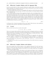
and credit risk. Consider the cash flow diagram in Figure 1-1. Here, the time is continuous and
the t0 , t1 , t2 represent some specific dates. Initially we place ourselves at time t0 . The following
deal is struck with a bank. At time t1 we borrow USD100, at the going interest rate of time
t1 , called the Libor and denoted by the symbol Lt1 . We pay the interest and the principal back
at time t2 . The loan has no default risk and is for a period of δ units of time.1 Note that the
contract is written at time t0 , but starts at the future date t1 . Hence this is an example of forward
contracts. The actual value of Lt1 will also be determined at the future date t1 .
Now, consider the time interval from t0 to t1 , expressed as t ∈ [t0 , t1 ]. At any time during
this interval, what can we say about the value of this forward contract initiated at t0 ?
It turns out that this contract will have a value identically equal to zero for all t ∈ [t0 , t1 ]
regardless of what happens in world financial markets. Perceptions of future interest rate

1 The δ is measured in proportion to a year. For example, assuming that a “year” is 360 days and a “month” is
always 30 days, a 3-month loan will give δ = 14 .

1


2

C

H A P T E R

. Introduction

1

Proceeds received

1 100
Interest and
Principal paid

t0

t1

t2
2Lt d100
1

2 100
Contract
initiation

FIGURE 1-1

movements may go from zero to infinity, but the value of the contract will still remain zero. In
order to prove this assertion, we calculate the value of the contract at time t0 . Actually, the value
is obvious in one sense. Look at Figure 1-1. No cash changes hand at time t0 . So, the value of
the contract at time t0 must be zero. This may be obvious but let us show it formally.
To value the cash flows in Figure 1-1, we will calculate the time t1 -value of the cash flows
that will be exchanged at time t2 . This can be done by discounting them with the proper discount
factor. The best discounting is done using the Lt1 itself, although at time t0 the value of this
Libor rate is not known. Still, the time t1 value of the future cash flows are
P Vt1 =

100
Lt1 δ100
+
(1 + Lt1 δ) (1 + Lt1 δ)

(1)

At first sight it seems we would need an estimate of the random variable Lt1 to obtain a numerical
answer from this formula. In fact some market practitioners may suggest using the corresponding
forward rate that is observed at time t0 in lieu of Lt1 , for example. But a closer look suggests a
much better alternative. Collecting the terms in the numerator
P Vt1 =

(1 + Lt1 δ)100
(1 + Lt1 δ)

(2)

the unknown terms cancel out and we obtain:
P Vt1 = 100

(3)

This looks like a trivial result, but consider what it means. In order to calculate the value of the
cash flows shown in Figure 1-1, we don’t need to know Lt1 . Regardless of what happens to
interest rate expectations and regardless of market volatility, the value of these cash flows, and
hence the value of this contract, is always equal to zero for any t ∈ [t0 , t1 ]. In other words, the
price volatility of this instrument is identically equal to zero.
This means that given any instrument at time t, we can add (or subtract) the Libor loan to it,
and the value of the original instrument will not change for all t ∈ [t0 , t1 ]. We now apply this

simple idea to a number of basic operations in financial markets.

1.1. Buying a Default-Free Bond
For many of the operations they need, market practitioners do not “buy” or “sell” bonds. There
is a much more convenient way of doing business.


1. A Unique Instrument

3

1100
1rt d100
0

t0

t1

t2

Receive interest
and principal
2100
Pay cash

FIGURE 1-2. Buying default-free bond.

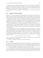
The cash flows of buying a default-free coupon bond with par value 100 forward are shown
in Figure 1-2. The coupon rate, set at time t0 , is rt0 . The price is USD100, hence this is a par

bond and the maturity date is t2 . Note that this implies the following equality:
100 =

rt0 δ100
100
+
(1 + rt0 δ) (1 + rt0 δ)

(4)

which is true, because at t0 , the buyer is paying USD100 for the cash flows shown in Figure 1-2.
Buying (selling) such a bond is inconvenient in many respects. First, one needs cash to do
this. Practitioners call this funding, in case the bond is purchased. When the bond is sold short
it will generate new cash and this must be managed.2 Hence, such outright sales and purchases
require inconvenient and costly cash management.
Second, the security in question may be a registered bond, instead of being a bearer bond,
whereas the buyer may prefer to stay anonymous.
Third, buying (selling) the bond will affect balance sheets, called books in the industry.
Suppose the practitioner borrows USD100 and buys the bond. Both the asset and the liability
sides of the balance sheet are now larger. This may have regulatory implications.3
Finally, by securing the funding, the practitioner is getting a loan. Loans involve credit risk.
The loan counterparty may want to factor a default risk premium into the interest rate.4
Now consider the following operation. The bond in question is a contract. To this contract “add” the forward Libor loan that we discussed in the previous section. This is shown in
Figure 1-3a. As we already proved, for all t ∈ [t0 , t1 ], the value of the Libor loan is identically
equal to zero. Hence, this operation is similar to adding zero to a risky contract. This addition
does not change the market risk characteristics of the original position in any way. On the other
hand, as Figure 1-3a and 1-3b show, the resulting cash flows are significantly more convenient
than the original bond.
The cash flows require no upfront cash, they do not involve buying a registered security,
and the balance sheet is not affected in any way. Yet, the cash flows shown in Figure 1-3 have

exactly the same market risk characteristics as the original bond.
Since the cash flows generated by the bond and the Libor loan in Figure 1-3 accomplish the
same market risk objectives as the original bond transaction, then why not package them as a
separate instrument and market them to clients under a different name? This is an Interest Rate

2

Short selling involves borrowing the bond and then selling it. Hence, there will be a cash management issue.

3 For example, this was an emerging market or corporate bond, the bank would be required to hold additional capital
against this purchase.
4

If the Treasury security being purchased is left as collateral, then this credit risk aspect mostly disappears.


4

C

H A P T E R

. Introduction

1

(a)

1100
1Lt d100

0

t0

t1

t2

2100
1100

t0

t1

t2

2Lt d100
1

2100

(b)
1st

Add vertically

0

d100

Received fixed

Interest
rate
swap

t0

t1

t2

Pay floating
2L t

1

d100

FIGURE 1-3

Swap (IRS). The party is paying a fixed rate and receiving a floating rate. The counterparty is
doing the reverse. IRSs are among the most liquid instruments in financial markets.

1.2. Buying Stocks
Suppose now we change the basic instrument. A market practitioner would like to buy a stock St
at time t0 with a t1 delivery date. We assume that the stock does not pay dividends. Hence, this
is, again, a forward purchase. The stock position will be liquidated at time t2 . Also, assume that
the time-t0 perception of the stock market gains or losses is such that the markets are demanding
a price

St0 = 100

(5)

for this stock as of time t0 . This situation is shown in Figure 1-4a, where the ΔSt2 is the unknown
stock price appreciation or depreciation to be observed at time t2 . Note that the original price


1. A Unique Instrument

(a)

5

1100
DSt

t0

2

t1

t2
DSt

2100

2

(If Iosses)

(Note the there
will be either
gains or losses, not
both as shown in
the graph)

1100

t0

t1

t2
2Lt d100
1

2100

(b)
Equity and commodity swap

t0

Receive any gains

t1

t2

Pay Libor and
any losses
Pay if losses DS t

2

Libor

FIGURE 1-4

being 100, the time t2 stock price can be written as
St2 = St1 + ΔSt2
= 100 + ΔSt2

(6)

Hence the cash flows shown in Figure 1-4a.
It turns out that whatever the purpose of buying such a stock was, this outright purchase
suffers from even more inconveniences than in the case of the bond. Just as in the case of
the Treasury bond, the purchase requires cash, is a registered transaction with significant tax
implications, and immediately affects the balance sheets, which have regulatory implications.
A fourth inconvenience is a very simple one. The purchaser may not be allowed to own such a
stock.5 Last, but not least, there are regulations preventing highly leveraged stock purchases.
Now, apply the same technique to this transaction. Add the Libor loan to the cash flows
shown in Figure 1-4a and obtain the cash flows in Figure 1-4b. As before, the market risk

5

For example, only special foreign institutions are allowed to buy Chinese A-shares that trade in Shanghai.

6

C

H A P T E R

. Introduction

1

characteristics of the portfolio are identical to those of the original stock. The resulting cash
flows can be marketed jointly as a separate instrument. This is an equity swap and it has none
of the inconveniences of the outright purchase. But, because we added a zero to the original
cash flows, it has exactly the same market risk characteristics as a stock. In an equity swap, the
party is receiving any stock market gains and paying a floating Libor rate plus any stock market
losses.6
Note that if St denoted the price of any commodity, such as oil, then the same logic would
give us a commodity swap.7

1.3. Buying a Defaultable Bond
Consider the bond in Figure 1-1 again, but this time assume that at time t2 the issuer can default.
The bond pays the coupon ct0 with
rt0 < ct0
(7)
where rt0 is a risk-free rate. The bond sells at par value, USD100 at time t0 . The interest and
principal are received at time t2 if there is no default. If the bond issuer defaults the investor
receives nothing. This means that we are working with a recovery rate of zero. Figure 1-5a
shows this characterization.

(a)

1100
Ct d100
0

t0

t1

No default

t2

2100
Default

t2
(b)

1100

Libor loan

t0

t1

t2

2Lt d100
1

2100

FIGURE 1-5

6 If stocks decline at the settlement times, the investor will pay the Libor indexed cash flows and the loss in the
stock value.
7 To be exact, this commodity should have no other payout or storage costs associated with it, it should not have any
convenience yield either. Otherwise the swap structure will change slightly. This is equivalent to assuming no dividend
payments and will be discussed in Chapter 3.


1. A Unique Instrument

7

This transaction has, again, several inconveniences. In fact, all the inconveniences mentioned
there are still valid. But, in addition, the defaultable bond may not be very liquid.8 Also, because
it is defaultable, the regulatory agencies will certainly impose a capital charge on these bonds if
they are carried on the balance sheet.
A much more convenient instrument is obtained by adding the “zero” to the defaultable
bond and forming a new portfolio. Visualized together with a Libor loan, the cash flows of a
defaultable bond shown in Figure 1-5a change as shown in Figure 1-5b. But we can go one
step further in this case. Assume that at time t0 there is an interest rate swap (IRS) trading
actively in the market. Then we can add this interest rate swap to Figure 1-5b and obtain a much
clearer picture of the final cash flows. This operation is shown in Figure 1-6. In fact, this last
step eliminates the unknown future Libor rates Lti and replaces them with the known swap
rate st0 .

The resulting cash flows don’t have any of the inconveniences suffered by the defaultable
bond purchase. Again, they can be packaged and sold separately as a new instrument. Letting the
st0 denote the rate on the corresponding interest rate swap, the instrument requires receipts of
a known and constant premium ct0 − st0 periodically. Against this a floating (contingent) cash
flow is paid. In case of default, the counterparty is compensated by USD100. This is similar
to buying and selling default insurance. The instrument is called a credit default swap (CDS).
Since their initiation during the 1990s CDSs have become very liquid instruments and completely
changed the trading and hedging of credit risk. The insurance premium, called the CDS spread
cdst0 , is given by
cdst0 = ct0 − st0

(8)

This rate is positive since the ct0 should incorporate a default risk premium, which the defaultfree bond does not have.9

1Ct

0

No default

t0

t1

t2

2Lt

1

Default

2Lt

1

(Assuming d 5 1)

2100

FIGURE 1-6

8

Many corporate bonds do not trade in the secondary market at all.

9 The connection between the CDS rates and the differential c
t0 − st0 is more complicated in real life. Here we
are working within a simplified setup.


8

C

H A P T E R

. Introduction

1

1.4. First Conclusions
This section discussed examples of the first method of financial engineering. Switching from cash
transactions to trading various swaps has many advantages. By combining an instrument with a
forward Libor loan contract in a specific way, and then selling the resulting cash flows as separate
swap contracts, the financial engineer has succeeded in accomplishing the same objectives much
more efficiently and conveniently. The resulting swaps are likely to be more efficient, cost
effective and liquid than the underlying instruments. They also have better regulatory and tax
implications.
Clearly, one can sell as well as buy such swaps. Also, one can reverse engineer the bond,
equity, and the commodities by combining the swap with the Libor deposit. Chapter 5 will
generalize this swap engineering. In the next section we discuss another major financial engineering principle: the way one can build synthetic instruments.
We now introduce some simple financial engineering strategies. We consider two examples
that require finding financial engineering solutions to a daily problem. In each case, solving
the problem under consideration requires creating appropriate synthetics. In doing so, legal,
institutional, and regulatory issues need to be considered.
The nature of the examples themselves is secondary here. Our main purpose is to bring to
the forefront the way of solving problems using financial securities and their derivatives. The
chapter does not go into the details of the terminology or of the tools that are used. In fact, some
readers may not even be able to follow the discussion fully. There is no harm in this since these
will be explained in later chapters.

2.

A Money Market Problem
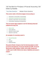
Consider a Japanese bank in search of a 3-month money market loan. The bank would like
to borrow U.S. dollars (USD) in Euromarkets and then on-lend them to its customers. This
interbank loan will lead to cash flows as shown in Figure 1-7. From the borrower’s angle,
USD100 is received at time t0 , and then it is paid back with interest 3 months later at time

t0 + δ. The interest rate is denoted by the symbol Lt0 and is determined at time t0 . The tenor of
the loan is 3 months. Therefore
1
(9)
δ=
4
and the interest paid becomes Lt0 14 . The possibility of default is assumed away.10

Cash inflow
1100 USD

t0

Cash outflow

t1 5 t01 d
t1
2100 (1 1 Lt d)
0

Borrow
(Receive USD)

Pay back
with interest

FIGURE 1-7. A USD loan.

10

Otherwise at time t0 + δ there would be a conditional cash outflow depending on whether or not there is default.


2. A Money Market Problem

9

The money market loan displayed in Figure 1-7 is a fairly liquid instrument. In fact, banks
purchase such “funds” in the wholesale interbank markets, and then on-lend them to their
customers at a slightly higher rate of interest.

2.1. The Problem
Now, suppose the above-mentioned Japanese bank finds out that this loan is not available due to
the lack of appropriate credit lines. The counterparties are unwilling to extend the USD funds.
The question then is: Are there other ways in which such dollar funding can be secured?
The answer is yes. In fact, the bank can use foreign currency markets judiciously to construct
exactly the same cash flow diagram as in Figure 1-7 and thus create a synthetic money market
loan. The first cash flow is negative and is placed below the time axis because it is a payment
by the investor. The subsequent sale of the asset, on the other hand, is a receipt, and hence is
represented by a positive cash flow placed above the time axis. The investor may have to pay
significant taxes on these capital gains. A relevant question is then: Is it possible to use a strategy
that postpones the investment gain to the next tax year? This may seem an innocuous statement,
but note that using currency markets and their derivatives will involve a completely different
set of financial contracts, players, and institutional setup than the money markets. Yet, the result
will be cash flows identical to those in Figure 1-7.

2.2. Solution
To see how a synthetic loan can be created, consider the following series of operations:
1. The Japanese bank first borrows local funds in yen in the onshore Japanese money markets.
This is shown in Figure 1-8a. The bank receives yen at time t0 and will pay yen interest

rate LYt0 δ at time t0 + δ.
2. Next, the bank sells these yen in the spot market at the current exchange rate et0 to secure
USD100. This spot operation is shown in Figure 1-8b.
3. Finally, the bank must eliminate the currency mismatch introduced by these operations.
In order to do this, the Japanese bank buys 100(1 + Lt0 δ)ft0 yen at the known forward
exchange rate ft0 , in the forward currency markets. This is the cash flow shown in
Figure 1-8c. Here, there is no exchange of funds at time t0 . Instead, forward dollars will
be exchanged for forward yen at t0 + δ.
Now comes the critical point. In Figure 1-8, add vertically all the cash flows generated by
these operations. The yen cash flows will cancel out at time t0 because they are of equal size and
different sign. The time t0 + δ yen cash flows will also cancel out because that is how the size
of the forward contract is selected. The bank purchases just enough forward yen to pay back the
local yen loan and the associated interest. The cash flows that are left are shown in Figure 1-8d,
and these are exactly the same cash flows as in Figure 1-7. Thus, the three operations have
created a synthetic USD loan. The existence of the FX-forward played a crucial role in this
synthetic.

2.3. Some Implications
There are some subtle but important differences between the actual loan and the synthetic. First,
note that from the point of view of Euromarket banks, lending to Japanese banks involves a
principal of USD100, and this creates a credit risk. In case of default, the 100 dollars lent may
not be repaid. Against this risk, some capital has to be put aside. Depending on the state of money


10

C

H A P T E R

. Introduction

1

(a)

Borrow
yen...

t0

t1
Pay borrowed yen
1 interest
1

(b)

USD

t0

t1

Buy spot dollars
with the yen...
1

(c)

1Yen

t0
...Buy the needed yen forward.

t1
2USD

Adding vertically, yen cash flows cancel...
(d)

USD

t0

t1
2USD

The result is like a USD loan.

FIGURE 1-8. A synthetic USD loan.

markets and depending on counterparty credit risks, money center banks may adjust their credit
lines toward such customers.
On the other hand, in the case of the synthetic dollar loan, the international bank’s exposure
to the Japanese bank is in the forward currency market only. Here, there is no principal involved.
If the Japanese bank defaults, the burden of default will be on the domestic banking system in
Japan. There is a risk due to the forward currency operation, but it is a counterparty risk and
is limited. Thus, the Japanese bank may end up getting the desired funds somewhat easier if a
synthetic is used.

There is a second interesting point to the issue of credit risk mentioned earlier. The original
money market loan was a Euromarket instrument. Banking operations in Euromarkets are considered offshore operations, taking place essentially outside the jurisdiction of national banking
authorities. The local yen loan, on the other hand would be subject to supervision by Japanese
authorities, obtained in the onshore market. In case of default, there may be some help from
the Japanese Central Bank, unlike a Eurodollar loan where a default may have more severe
implications on the lending bank.


3. A Taxation Example

11

The third point has to do with pricing. If the actual and synthetic loans have identical cash
flows, their values should also be the same excluding credit risk issues. If there is a value
discrepancy the markets will simultaneously sell the expensive one, and buy the cheaper one,
realizing a windfall gain. This means that synthetics can also be used in pricing the original
instrument.11
Fourth, note that the money market loan and the synthetic can in fact be each other’s hedge.
Finally, in spite of the identical nature of the involved cash flows, the two ways of securing dollar
funding happen in completely different markets and involve very different financial contracts.
This means that legal and regulatory differences may be significant.

3.

A Taxation Example
Now consider a totally different problem. We create synthetic instruments to restructure taxable
gains. The legal environment surrounding taxation is a complex and ever-changing phenomenon,
therefore this example should be read only from a financial engineering perspective and not as a
tax strategy. Yet the example illustrates the close connection between what a financial engineer
does and the legal and regulatory issues that surround this activity.

3.1. The Problem
In taxation of financial gains and losses, there is a concept known as a wash-sale. Suppose that
during the year 2007, an investor realizes some financial gains. Normally, these gains are taxable
that year. But a variety of financial strategies can possibly be used to postpone taxation to the year
after. To prevent such strategies, national tax authorities have a set of rules known as wash-sale
and straddle rules. It is important that professionals working for national tax authorities in various
countries understand these strategies well and have a good knowledge of financial engineering.
Otherwise some players may rearrange their portfolios, and this may lead to significant losses
in tax revenues. From our perspective, we are concerned with the methodology of constructing
synthetic instruments.
Suppose that in September 2007, an investor bought an asset at a price S0 = $100. In December 2007, this asset is sold at S1 = $150. Thus, the investor has realized a capital gain of $50.
These cash flows are shown in Figure 1-9.

Dec. 2007
$50
Sept. 2007
Jan. 2007

Liquidate and
realize the
capital gains

$100
Jan. 2008

invest 2$100

FIGURE 1-9. An investment liquidated on Dec. 2007.

11

However, the credit risk issues mentioned earlier may introduce a wedge between the prices of the two loans.


12

C

H A P T E R

. Introduction

1

One may propose the following solution. This investor is probably holding assets other than
the St mentioned earlier. After all, the right way to invest is to have diversifiable portfolios. It is
also reasonable to assume that if there were appreciating assets such as St , there were also assets
that lost value during the same period. Denote the price of such an asset by Zt . Let the purchase
price be Z0 . If there were no wash-sale rules, the following strategy could be put together to
postpone year 2007 taxes.
Sell the Z-asset on December 2007, at a price Z1 , Z1 < Z0 , and, the next day, buy the same
Zt at a similar price. The sale will result in a loss equal to
Z 1 − Z0 < 0

(10)

The subsequent purchase puts this asset back into the portfolio so that the diversified portfolio
can be maintained. This way, the losses in Zt are recognized and will cancel out some or all of
the capital gains earned from St . There may be several problems with this strategy, but one is

fatal. Tax authorities would call this a wash-sale (i.e., a sale that is being intentionally used to
“wash” the 2007 capital gains) and would disallow the deductions.
3.1.1.

Another Strategy

Investors can find a way to sell the Z-asset without having to sell it in the usual way. This can
be done by first creating a synthetic Z-asset and then realizing the implicit capital losses using
this synthetic, instead of the Z-asset held in the portfolio.
Suppose the investor originally purchased the Z-asset at a price Z0 = $100 and that asset
is currently trading at Z1 = $50, with a paper loss of $50. The investor would like to recognize
the loss without directly selling this asset. At the same time, the investor would like to retain the
original position in the Z-asset in order to maintain a well-balanced portfolio. How can the loss
be realized while maintaining the Z-position and without selling the Zt ?
The idea is to construct a proper synthetic. Consider the following sequence of operations:
• Buy another Z-asset at price Z1 = $50 on November 26, 2007.
• Sell an at-the-money call on Z with expiration date December 30, 2007.
• Buy an at-the-money put on Z with the same expiration.
The specifics of call and put options will be discussed in later chapters. For those readers with
no background in financial instruments we can add a few words. Briefly, options are instruments
that give the purchaser a right. In the case of the call option, it is the right to purchase the
underlying asset (here the Z-asset) at a prespecified price (here $50). The put option is the
opposite. It is the right to sell the asset at a prespecified price (here $50). When one sells options,
on the other hand, the seller has the obligation to deliver or accept delivery of the underlying at
a prespecified price.
For our purposes, what is important is that short call and long put are two securities whose
expiration payoff, when added, will give the synthetic short position shown in Figure 1-10. By
selling the call, the investor has the obligation to deliver the Z-asset at a price of $50 if the call
holder demands it. The put, on the other hand, gives the investor the right to sell the Z-asset at
$50 if he or she chooses to do so.

The important point here is this: When the short call and the long put positions shown in
Figure 1-10 are added together, the result will be equivalent to a short position on stock Zt . In
fact, the investor has created a synthetic short position using options.
Now consider what happens as time passes. If Zt appreciates by December 30, the call
will be exercised. This is shown in Figure 1-11a. The call position will lose money, since the
investor has to deliver, at a loss, the original Z-stock that cost $100. If, on the other hand, the Zt


3. A Taxation Example

Gain

13

Long position
in Zt

Zt
Z1 5 50

Loss
Purchase another Z-asset

Gain

Long put
with strike 50

Zt
K 5 50

Loss

Short call
with strike 50

Strike
price
Synthetic short position in Z-asset

FIGURE 1-10. Two positions that cancel each other.

decreases, then the put position will enable the investor to sell the original Z-stock at $50. This
time the call will expire worthless.12 This situation is shown in Figure 1-11b. Again, there will
be a loss of $50. Thus, no matter what happens to the price Zt , either the investor will deliver
the original Z-asset purchased at a price $100, or the put will be exercised and the investor will
sell the original Z-asset at $50. Thus, one way or another, the investor is using the original asset
purchased at $100 to close an option position at a loss. This means he or she will lose $50 while
keeping the same Z-position, since the second Z, purchased at $50, will still be in the portfolio.
The timing issue is important here. For example, according to U.S. tax legislation, wash-sale
rules will apply if the investor has acquired or sold a substantially identical property within a 31day period. According to the strategy outlined here, the second Z is purchased on November 26,
while the options expire on December 30. Thus, there are more than 31 days between the two
operations.13

3.2. Implications
There are at least three interesting points to our discussion. First, the strategy offered to the
investor was risk-free and had zero cost aside from commissions and fees. Whatever happens

12
13

For technical reasons, suppose both options can be exercised only at expiration. They are of European style.

The timing considerations suggest that the strategy will be easier to apply if over-the-counter (OTC) options are
used, since the expiration dates of exchange-traded options may occur at specific dates, which may not satisfy the legal
timing requirements.


14

C

H A P T E R

. Introduction

1

(a) 1

If Zt appreciates short call will be exercised, with a loss of 50.

K 5 50

Z
Dec. 30

Zt

Receive $50,

deliver Z with cost $100.

2

Short call
Long put
(b) 1
If Zt declines, the put is exercised.
Z
Zt

Dec. 30

2

K 5 50

Receive $50,
deliver the Z with cost $100, the loss is again 50.

FIGURE 1-11. The strategy with the Z initially at 50. Two ways to realize loss.

to the new long position in the Z-asset, it will be canceled by the synthetic short position.
This situation is shown in the lower half of Figure 1-10. As this graph shows, the proposed
solution has no market risk, but may have counterparty, or operational risks. The second point
is that, once again, we have created a synthetic, and then used it in providing a solution to our
problem. Finally, the example displays the crucial role legal and regulatory frameworks can
play in devising financial strategies. Although this book does not deal with these issues, it is
important to understand the crucial role they play at almost every level of financial engineering.

4.

Some Caveats for What Is to Follow
A newcomer to financial engineering usually follows instincts that are harmful for good understanding of the basic methodologies in the field. Hence, before we start, we need to lay out some
basic rules of the game that should be remembered throughout the book.
1. This book is written from a market practitioner’s point of view. Investors, pension funds,
insurance companies, and governments are clients, and for us they are always on the other
side of the deal. In other words, we look at financial engineering from a trader’s, broker’s,
and dealer’s angle. The approach is from the manufacturer’s perspective rather than the
viewpoint of the user of the financial services. This premise is crucial in understanding
some of the logic discussed in later chapters.


5. Trading Volatility

15

2. We adopt the convention that there are two prices for every instrument unless stated
otherwise. The agents involved in the deals often quote two-way prices. In economic
theory, economic agents face the law of one price. The same good or asset cannot have
two prices. If it did, we would then buy at the cheaper price and sell at the higher price.
Yet for a market maker, there are two prices: one price at which the market participant
is willing to buy something from you, and another one at which the market participant is
willing to sell the same thing to you. Clearly, the two cannot be the same. An automobile
dealer will buy a used car at a low price in order to sell it at a higher price. That is how
the dealer makes money. The same is true for a market practitioner. A swap dealer will
be willing to buy swaps at a low price in order to sell them at a higher price later. In the
meantime, the instrument, just like the used car sold to a car dealer, is kept in inventories.
3. It is important to realize that a financial market participant is not an investor and never
has “money.” He or she has to secure funding for any purchase and has to place the cash

generated by any sale. In this book, almost no financial market operation begins with a
pile of cash. The only “cash” is in the investor’s hands, which in this book is on the other
side of the transaction.
It is for this reason that market practitioners prefer to work with instruments that have
zero-value at the time of initiation. Such instruments would not require funding and are
more practical to use.14 They also are likely to have more liquidity.
4. The role played by regulators, professional organizations, and the legal profession is much
more important for a market professional than for an investor. Although it is far beyond
the scope of this book, many financial engineering strategies have been devised for the
sole purpose of dealing with them.
Remembering these premises will greatly facilitate the understanding of financial engineering.

5.

Trading Volatility
Practitioners or investors can take positions on expectations concerning the price of an asset.
Volatility trading involves positions taken on the volatility of the price. This is an attractive
idea, but how does one buy or sell volatility? Answering this question will lead to a third basic
methodology in financial engineering. This idea is a bit more complicated, so the argument
here will only be an introduction. Chapter 8 will present a more detailed treatment of the
methodology.
In order to discuss volatility trading, we need to introduce the notion of convexity gains.
We start with a forward contract. Let us stay within the framework of the previous section and
assume that Ft0 is the forward dollar-yen exchange rate.15 Suppose at time t0 we take a long
position in the U.S. dollar as shown in Figure 1-15. The upward sloping line is the so-called
payoff function.16 For example, if at time t0 + Δ the forward price becomes Ft0 +Δ , we can
close the position with a gain:
(11)
gain = Ft0 +Δ − Ft0
It is important, for the ensuing discussion, that this payoff function be a straight line with a

constant slope.

14

Although one could pay bid-ask spreads or commissions during the process.

15

The et0 denotes the spot exchange rate USD/JPY, which is the value of one dollar in terms of Japanese yen at
time t0 .
16 Depending on at what point the spot exchange rate denoted by e , ends up at time T , we either gain or lose from
T
this long position.