John wiley sons exploratory data mining data cleaning (2003)

Exploratory Data Mining
and Data Cleaning


WILEY SERIES IN PROBABILITY AND STATISTICS
Established by WALTER A. SHEWHART and SAMUEL S. WILKS
Editors: David J. Balding, Peter Bloomfield, Noel A. C. Cressie,
Nicholas I. Fisher, Iain M. Johnstone, J. B. Kadane, Louise M. Ryan,
David W. Scott, Adrian F. M. Smith, Jozef L. Teugels;
Editors Emeriti: Vic Barnett, J. Stuart Hunter, David G. Kendall
A complete list of the titles in this series appears at the end of this volume.


Exploratory Data Mining
and Data Cleaning
TAMRAPARNI DASU
THEODORE JOHNSON
AT&T Labs, Research Division
Florham Park, NJ

A JOHN WILEY & SONS, INC., PUBLICATION


Copyright © 2003 by John Wiley & Sons, Inc. All rights reserved.
Published by John Wiley & Sons, Inc., Hoboken, New Jersey.
Published simultaneously in Canada.
No part of this publication may be reproduced, stored in a retrieval system, or transmitted in any
form or by any means, electronic, mechanical, photocopying, recording, scanning, or otherwise,
except as permitted under Section 107 or 108 of the 1976 United States Copyright Act, without
either the prior written permission of the Publisher, or authorization through payment of the

appropriate per-copy fee to the Copyright Clearance Center, Inc., 222 Rosewood Drive, Danvers,
MA 01923, 978-750-8400, fax 978-750-4470, or on the web at www.copyright.com. Requests to the
Publisher for permission should be addressed to the Permissions Department, John Wiley & Sons,
Inc., 111 River Street, Hoboken, NJ 07030, (201) 748-6011, fax (201) 748-6008, e-mail:

Limit of Liability/Disclaimer of Warranty: While the publisher and author have used their best
efforts in preparing this book, they make no representations or warranties with respect to the
accuracy or completeness of the contents of this book and specifically disclaim any implied warranties of merchantability or fitness for a particular purpose. No warranty may be created or
extended by sales representatives or written sales materials. The advice and strategies contained
herein may not be suitable for your situation. You should consult with a professional where appropriate. Neither the publisher nor author shall be liable for any loss of profit or any other commercial damages, including but not limited to special, incidental, consequential, or other damages.
For general information on our other products and services please contact our Customer Care
Department within the U.S. at 877-762-2974, outside the U.S. at 317-572-3993 or fax 317-572-4002.
Wiley also publishes its books in a variety of electronic formats. Some content that appears in
print, however, may not be available in electronic format.
Library of Congress Cataloging-in-Publication Data:
Dasu, Tamraparni.
Exploratory data mining and data cleaning / Tamraparni Dasu, Theorodre Johnson.
p. cm.
Includes bibliographical references and index.
ISBN 0-471-26851-8 (cloth)
1. Data mining. 2. Electronic data processing—Data preparation. 3. Electronic data
processing—Quality control. I. Johnson, Theodore. II. Title.
QA76.9.D343 D34 2003
006.3—dc21
2002191085
Printed in the United States of America.
10 9 8 7 6 5 4 3 2 1


Contents

Preface

ix

1. Exploratory Data Mining and Data Cleaning: An Overview

1

1.1
1.2
1.3
1.4
1.5
1.6

1.7

1.8

Introduction, 1
Cautionary Tales, 2
Taming the Data, 4
Challenges, 4
Methods, 6
EDM, 7
1.6.1 EDM Summaries—Parametric, 8
1.6.2 EDM Summaries—Nonparametric, 9
End-to-End Data Quality (DQ), 12
1.7.1 DQ in Data Preparation, 13

1.7.2 EDM and Data Glitches, 13
1.7.3 Tools for DQ, 14
1.7.4 End-to-End DQ: The Data Quality Continuum, 14
1.7.5 Measuring Data Quality, 15
Conclusion, 16

2. Exploratory Data Mining
2.1
2.2
2.3
2.4

17

Introduction, 17
Uncertainty, 19
2.2.1 Annotated Bibliography, 23
EDM: Exploratory Data Mining, 23
EDM Summaries, 25
2.4.1 Typical Values, 26
2.4.2 Attribute Variation, 33
v


vi

contents
2.4.3 Example, 41
2.4.4 Attribute Relationships, 42
2.4.5 Annotated Bibliography, 49

2.5 What Makes a Summary Useful?, 50
2.5.1 Statistical Properties, 51
2.5.2 Computational Criteria, 54
2.5.3 Annotated Bibliography, 54
2.6 Data-Driven Approach—Nonparametric Analysis, 54
2.6.1 The Joy of Counting, 55
2.6.2 Empirical Cumulative Distribution Function (ECDF), 57
2.6.3 Univariate Histograms, 59
2.6.4 Annotated Bibliography, 61
2.7 EDM in Higher Dimensions, 62
2.8 Rectilinear Histograms, 62
2.9 Depth and Multivariate Binning, 64
2.9.1 Data Depth, 65
2.9.2 Aside: Depth-Related Topics, 66
2.9.3 Annotated Bibliography, 68
2.10 Conclusion, 68

3. Partitions and Piecewise Models
3.1

3.2
3.3
3.4

3.5

Divide and Conquer, 69
3.1.1 Why Do We Need Partitions?, 70
3.1.2 Dividing Data, 71
3.1.3 Applications of Partition-Based EDM Summaries, 73

Axis-Aligned Partitions and Data Cubes, 74
3.2.1 Annotated Bibliography, 77
Nonlinear Partitions, 77
3.3.1 Annotated Bibliography, 78
DataSpheres (DS), 78
3.4.1 Layers, 79
3.4.2 Data Pyramids, 81
3.4.3 EDM Summaries, 82
3.4.4 Annotated Bibliography, 82
Set Comparison Using EDM Summaries, 82
3.5.1 Motivation, 83
3.5.2 Comparison Strategy, 83
3.5.3 Statistical Tests for Change, 84

69


contents

3.6

3.7

3.8

3.9

vii
3.5.4 Application—Two Case Studies, 85
3.5.5 Annotated Bibliography, 88

Discovering Complex Structure in Data with EDM
Summaries, 89
3.6.1 Exploratory Model Fitting in Interactive Response
Time, 89
3.6.2 Annotated Bibliography, 90
Piecewise Linear Regression, 90
3.7.1 An Application, 92
3.7.2 Regression Coefficients, 92
3.7.3 Improvement in Fit, 94
3.7.4 Annotated Bibliography, 94
One-Pass Classification, 95
3.8.1 Quantile-Based Prediction with Piecewise Models, 95
3.8.2 Simulation Study, 96
3.8.3 Annotated Bibliography, 98
Conclusion, 98

4. Data Quality
4.1
4.2

4.3

4.4

Introduction, 99
The Meaning of Data Quality, 102
4.2.1 An Example, 102
4.2.2 Data Glitches, 103
4.2.3 Conventional Definition of DQ, 105
4.2.4 Times Have Changed, 106

4.2.5 Annotated Bibliography, 108
Updating DQ Metrics: Data Quality Continuum, 108
4.3.1 Data Gathering, 109
4.3.2 Data Delivery, 110
4.3.3 Data Monitoring, 113
4.3.4 Data Storage, 116
4.3.5 Data Integration, 118
4.3.6 Data Retrieval, 120
4.3.7 Data Mining/Analysis, 121
4.3.8 Annotated Bibliography, 123
The Meaning of Data Quality Revisited, 123
4.4.1 Data Interpretation, 124
4.4.2 Data Suitability, 124
4.4.3 Dataset Type, 124

99


viii

contents

4.5

4.6
4.7

4.4.4 Attribute Type, 128
4.4.5 Application Type, 129
4.4.6 Data Quality—A Many Splendored Thing, 129

4.4.7 Annotated Bibliography, 130
Measuring Data Quality, 130
4.5.1 DQ Components and Their Measurement, 131
4.5.2 Combining DQ Metrics, 134
The DQ Process, 134
Conclusion, 136
4.7.1 Four Complementary Approaches, 136
4.7.2 Annotated Bibliography, 137

5. Data Quality: Techniques and Algorithms
5.1
5.2

5.3

5.4

5.5

5.6

139

Introduction, 139
DQ Tools Based on Statistical Techniques, 140
5.2.1 Missing Values, 141
5.2.2 Incomplete Data, 144
5.2.3 Outliers, 146
5.2.4 Detecting Glitches Using Set Comparison, 151
5.2.5 Time Series Outliers: A Case Study, 154

5.2.6 Goodness-of-Fit, 160
5.2.7 Annotated Bibliography, 161
Database Techniques for DQ, 162
5.3.1 What is a Relational Database?, 162
5.3.2 Why Are Data Dirty?, 165
5.3.3 Extraction, Transformation, and Loading (ETL), 166
5.3.4 Approximate Matching, 168
5.3.5 Database Profiling, 172
5.3.6 Annotated Bibliography, 175
Metadata and Domain Expertise, 176
5.4.1 Lineage Tracing, 179
5.4.2 Annotated Bibliography, 179
Measuring Data Quality?, 180
5.5.1 Inventory Building—A Case Study, 180
5.5.2 Learning and Recommendations, 186
Data Quality and Its Challenges, 188

Bibliography

189

Index

197


Preface

As data analysts at a large information-intensive business, we often have been
asked to analyze new (to us) data sets. This experience was the original motivation for our interest in the topics of exploratory data mining and data

quality. Most data mining and analysis techniques assume that the data have
been joined into a single table and cleaned, and that the analyst already knows
what she or he is looking for. Unfortunately, the data set is usually dirty,
composed of many tables, and has unknown properties. Before any results
can be produced, the data must be cleaned and explored—often a long and
difficult task.
Current books on data mining and analysis usually focus on the last stage
of the analysis process (getting the results) and spend little time on how data
exploration and cleaning is done. Usually, their primary aim is to discuss the
efficient implementation of the data mining algorithms and the interpretation
of the results. However, the true challenges in the task of data mining are:
•

•

Creating a data set that contains the relevant and accurate information,
and
Determining the appropriate analysis techniques.

In our experience, the tasks of exploratory data mining and data cleaning constitute 80% of the effort that determines 80% of the value of the ultimate data
mining results. Data mining books (a good one is [56]) provide a great amount
of detail about the analytical process and advanced data mining techniques.
However they assume that the data has already been gathered, cleaned,
explored, and understood.
As we gained experience with exploratory data mining and data quality
issues, we became involved in projects in which data quality improvement was
the goal of the project (i.e., for operational databases) rather than a prerequisite. Several books recently have been published on the topic of ensuring data quality (e.g., the books by Loshin [84], by Redman [107]), and by
English [41]). However, these books are written for managers and take a
ix

x

preface

managerial viewpoint. While the problem of ensuring data quality requires a
significant managerial support, there is also a need for technical and analytic
tools. At the time of this writing, we have not seen any organized exposition
of the technical aspects of data quality management. The most closely related
book is Pyle [102], which discusses data preparation for data mining. However,
this text has little discussion of data quality issues or of exploratory data
mining—pre-requisites even to preparing data for data mining.
Our focus in this book is to develop a systematic process of data exploration and data quality management. We have found these seemingly unrelated topics to be inseparable. The exploratory phase of any data analysis
project inevitably involves sorting out data quality problems, and any data
quality improvement project inevitably involves data exploration. As a further
benefit, data exploration sheds light on appropriate analytic strategies.
Data quality is a notoriously messy problem that refuses to be put into a
neat container, and therefore is often viewed as technically intractable. We
have found that data quality problems can be addressed, but doing so requires
that we draw on methods from many disciplines: statistics, exploratory data
mining (EDM), databases, management, and metadata. Our focus in this book
is to present an integrated approach to EDM and data quality. Because of the
very broad nature of the subject, the exposition tends to be a summarization
of material discussed in great detail elsewhere (for which we provide references), with an emphasis on how the techniques relate to each other and to
EDM and data quality. Some topics (such as data quality metrics and certain
aspects of EDM) have no other good source, so we discuss them in greater
detail.

EXPLORATORY DATA MINING (EDM)
Data sets of the twenty-first century are different from the ones that motivated analytical techniques of statistics, machine learning and others. Earlier

data sets were reasonably small and relatively homogeneous so that the structure in them could be captured with compact models that had large but a manageable number of parameters. Many researchers have focused on scaling the
methods to run efficiently and quickly on the much larger data sets collected
by automated devices. In addition, methods have been developed specifically
for massive data (i.e., data mining techniques). However, there are two
fundamental issues that need to be addressed before these methods can be
applied.
•

A “data set” is often a patchwork of data collected from many sources,
which might not have been designed for integration. One example of this
problem is when two corporate entities providing different services to a
common customer base merge to become a single entity. Another is when
different divisions of a “federation enterprise” need to merge their data


preface

•

xi

stores. In such situations, approximate matching heuristics are used to
combine the data. The resulting patchwork data set will have many data
quality issues that need to be addressed. The data are likely to contain
many other data glitches, and these need to be treated as well.
Data mining methods often do not focus on the “appropriateness of the
model for the data,” namely, goodness-of-fit. While finding the best model
in a given class of models is desirable, it is equally important to determine
the class of models that best fits the data.

There is no simple or single method for analyzing a complex, unfamiliar
data set. The task typically requires the sequential application of disparate
techniques, leveraging the additional information acquired at each stage to
converge to a powerful, accurate and fast method. The end-product is often a
“piecewise technique” where at each stage we might have had to adapt or
extend, to improvise on an existing method. The importance of such an
approach has been emphasized by statisticians such as John Tukey [123] and
more recently in the machine learning community, for instance, in the AutoClass project [19].

DATA QUALITY
A major confounding factor in EDM is the presence of data quality issues.
These are often unearthed as “interesting patterns” but on closer examination
prove to be artifacts. We emphasize this aspect in our case study, since typically data analysts spend a significant portion of their time weeding-out data
quality problems. No matter how sophisticated the data mining techniques,
bad data will lead to misleading findings.
While most practitioners of data analysis are aware of the pitfalls of data
quality issues, it is only recently that there has been an emphasis on the systematic detection and removal of data problems. There have been efforts
directed at managing processes that generate the data, at cleaning up databases (e.g. merging/purging of duplicates), and at finding tools and algorithms
for the automatic detection of data glitches. Statistical methods for process
control (predominantly univariate) that date back to quality control charts
developed for detecting batches of poorly produced lots in industrial manufacturing are often adapted to monitor fluctuations in variables that populate
databases.
For operations databases, data quality is an end in itself. Most business (and
governmental, etc.) processes involve complex interactions between many
databases. Data quality problems can have very expensive manifestations (e.g.,
“losing” a cross-country cable, forgetting to bill customers). In this electronic
age, many businesses (and governmental organizations, etc.) would like to “eenable” their customers—that is, let them examine the relevant parts of the


xii

preface

operational databases to manage their own accounts. Depending on the state
of the underlying databases, this can be embarrassing or even impossible.

SUMMARY
In this book, we intend to:
•

•

•

•

Focus on developing a modeling strategy through an iterative data exploration loop and incorporation of domain knowledge;
Address methods for dealing with data quality issues that can have a
significant impact on findings and decisions, using commercially available
tools as well as new algorithmic approaches;
Emphasize application in real-life scenarios throughout the narrative with
examples;
Highlight new approaches and methodologies, such as the DataSphere
space partitioning and summary-based analysis techniques, and approaches to developing data quality metrics.

The book is intended for serious data analysts everywhere that need to
analyze large amounts of unfamiliar, potentially noisy data, and for managers
of operations databases. It can also serve as a text on data quality to supplement an advanced undergraduate or graduate level course in large-scale data
analysis and data mining. The book is especially appropriate for a crossdisciplinary course in statistics and computer science.

ACKNOWLEDGMENTS
We wish to thank the following people who have contributed to the material
in this book: Deepak Agarwal, Dave Belanger, Bob Bell, Simon Byers, Corinna
Cortes, Ken Church, Christos Faloutsos, Mary Fernandez, Joel Gottlieb,
Andrew Hume, Nick Koudas, Elefteris Koutsofios, Bala Krishnamurthy, Ken
Lyons, David Poole, Daryl Pregibon, Matthew Roughan, Gregg Vesonder, and
Jon Wright.


CHAPTER 1

Exploratory Data Mining and
Data Cleaning: An Overview

1.1 INTRODUCTION
Every data analysis task starts by gathering, characterizing, and cleaning a new,
unfamiliar data set. After this process, the data can be analyzed and the results
delivered. In our experience, the first step is far more difficult and time
consuming than the second. To start with, data gathering is a challenging task
complicated by problems both sociological (such as turf sensitivity) and
technological (different software and hardware platforms make transferring
and sharing data very difficult). Once the data are in place, acquiring the metadata (data descriptions, business rules) is another challenge. Very often the
metadata are poorly documented. When we finally are ready to analyze the
data, its quality is suspect. Furthermore, the data set is usually too large and
complex for manual inspection.
Sometimes, improved data quality is itself the goal of the analysis, usually
to improve processes in a production database (e.g., see the case study in
Section 5.5.1). Although the goal seems different than that of making an analysis, the methods and procedures are quite similar—in both cases we need to
understand the data, then take steps to improve data quality.
Fortunately, automated techniques can be applied to help understand the

data (Exploratory Data Mining, or EDM), and to help ensure data quality (by
data cleaning and applying data quality metrics). In this book we present these
techniques and show how they can be applied to prepare a data set for analysis. This chapter will briefly outline the challenges posed to the analysis of
massive data, the strategies for taming the data, and an overview of data exploration and cleaning methods, including developing meaningful data quality
definitions and metrics.

Exploratory Data Mining and Data Cleaning, by Tamraparni Dasu and Theodore Johnson
ISBN: 0-471-26851-8 Copyright © 2003 by John Wiley & Sons, Inc.

1


2

exploratory data mining and data cleaning

1.2 CAUTIONARY TALES
A first question to ask is, why are data exploration and data preparation
needed? Why not just go ahead and analyze the data? The answer is that the
results are almost guaranteed to be flawed. More specifically, some of the problems that occur are:
•

•

•

Spurious results: Data sets usually contain artifacts generated by external
sources that are of no interest to us but get mixed up with genuine
patterns of interest. For example, a study of traffic on a large telecommunications company’s data network revealed interesting behavior
over time. We were able to detect glitches caused by delays in gathering

and transmitting traffic characteristics (e.g., number of packets) and
remove such delays from inherent bursty patterns in the traffic. If we had
not cleaned the data, we would have included the glitches caused by
delays in the “signature usage pattern” of the customer, and would have
detected misleading deviations from the glitched signatures in future time
series.
Misplaced faith in black boxes: Data mining is sometimes perceived as a
black box, where you feed the data in and interesting results and patterns
emerge. Such an approach is particularly misleading when no prior
knowledge or experience is used to validate the results of the mining exercise. Consider the case of clustering, a method often used to find hidden
groupings in the data for tasks such as target marketing. It is very hard
to find good clusters without a reasonable estimate of the number of
groups, the relative sizes of these groups (e.g., cluster 1 is 10 times larger
than cluster 2) and the logic used by the clustering algorithm. For
example, if we use a k-means algorithm that initializes cluster centers at
random from the data, we need to choose at least 10 starting clusters to
detect two clusters that constitute 10% and 90% of the total data set.
Starting with fewer clusters would result in the algorithm finding one big
cluster containing most of the points, with a few outliers constituting the
other clusters.
Log-linear models (e.g., logistic regression) are another common
example of misplaced faith. The models are successful when the appropriate number of parameters and the correct explanatory variables are
included. The model will not fit well if too few parameters and irrelevant
variables are included in it, even if in reality the logistic regression model
is the correct choice. It is important to explore the data to arrive at an
appropriate analytical model.
Limitations of Popular Models: Very often, a model is chosen because it
is well understood or because the software is available, irrespective of the
nature of the data. Analysts rely on the robustness of the models, even
when underlying assumptions about the distribution (often the Normal

cautionary tales

•

3

density) do not hold. However, it is important to recognize that, although
classical parametric methods based on distributional and model assumptions are compact, powerful and accurate when used in the right conditions, they have limited applicability. They are not suitable for scenarios
where not enough is known about the data or its distribution, to validate
the assumptions of the classical methods. A good example is linear regression, which is often used inappropriately, because it is easy to use and
interpret. The underlying assumptions of linear effect of variables and the
form of error distributions are rarely verified. A random data set might
yield a linear regression model with a “reasonable” R-square goodnessof-fit measure, leading to a false confidence in the model.
Even if a model is applicable, it may be difficult to implement because
of the scale of the data. Many nonparametric methods, such as clustering,
machine learning, neural networks and others, are iterative and require
multiple passes over all the data. On very large data sets, they may be too
slow.
Buyer Beware—No Guarantees: Many data mining techniques do not
provide any goodness-of-fit guarantees. For example, a clustering mechanism might find the “best” clusters as defined by some distance metric,
but does not answer the question of how well the clusters replicate the
structure in the data. Testing the goodness-of-fit of clustering results with
respect to the data can be time consuming, involving simulation techniques. As a result, validation of clustering in the context of appropriateness to the data is often not implemented. The best or optimal model
could still be very poor at representing the underlying data. For example,
many financial firms (such as Long Term Capital Management) have
mined data sets to find similarities or differences in the prices of various
securities. In the case of LTCM, the analysts searched for securities whose
price tended to move in opposite directions and placed hedges by purchasing both. Unfortunately, these models proved to be inaccurate, and

LTCM lost billions of dollars when the price of the securities suddenly
moved in the same direction.
Another frequently encountered pitfall of casual data mining is spurious correlations. It is possible to find random time series that move
together over a period of time (e.g., the NASDAQ index and rainfall in
Bangladesh) but have no identifiable association, let alone causal relationship. An accompanying hazard is the tendency to tailor hypotheses
to the findings of a data mining exercise. A classical example is the
beer–diaper co-occurrence revealed by mining supermarket purchase
data. However, its not likely that one can increase beer sales by stocking
shelves with diapers.

We hope that the cautionary tales show that it is essential that the analyst must
clean and understand the data before analyzing it.


4

exploratory data mining and data cleaning

1.3 TAMING THE DATA
There are many books that address data analysis and model fitting in which a
single approach (logistic regression, neural networks) stands out as the method
of choice. In our experience, however, getting to the point where the modeling strategy is clear requires skill, science, and the lion’s share of the work. The
effectiveness of the later analysis strongly depends on the knowledge learned
during the earlier ground work. For an example, the analyst needs to know,
what are the variables that are relevant (e.g., for predicting probability of
recovery from a disease—vital statistics, past history, genetic propensity)? Of
these, how many variables can be measured and how many are a part of the
available data? How many are correlated and redundant? Which values are
suspicious and possibly inaccurate?
The work of identifying the final analysis strategy is an iterative (but computationally inexpensive) process alternating between exploratory data

mining (EDM) and data cleaning (improving data quality (DQ)). EDM consists of simple and fast summaries and analyses that reveal characteristics of
the data, such as typical values (averages, medians), variability (variance,
range), prevalence of different values (quantiles) and inter-relationships (correlations). During the course of EDM, certain data points that seem to be
unlikely (e.g., an outlier such as an 80-year-old third grader, a sign-up date of
08-31-95 for a service launched in 1997) motivate further investigation. Closer
scrutiny often finds data quality issues (a mistyped value, a system default
date), which, when fixed, result in cleaner, better quality data. In a later
chapter, we discuss a case study related to a provisioning data base where
clearing up data problems unearthed by EDM allowed us to significantly simplify the model needed to represent the structure in the data. We note that
addressing DQ issues involves consulting with domain experts and incorporating their knowledge into the next round of EDM. Therefore, EDM and DQ
have to be performed in conjunction.

1.4 CHALLENGES
Unfortunately, the analyst has to do considerable ground work before the
underlying structure in the data comes into focus. Some of the challenges of
EDM and DQ are:
•

Heterogeneity and Diversity: The data are often collected from many
sources and stitched together. This is particularly true of data gathered
from different organizations of a single “federation enterprise”, or of an
enterprise resulting from corporate mergers. Often, it is a problem even
for data gathered from different departments in the same organization.
The data might also be gathered from outside vendors (e.g., demographics). While the combined information is presented to the analyst as a


challenges

5

single data set, it usually contains a superposition of several statistical
processes. Analyzing such data using a single method or a black box
approach can produce misleading, if not totally incorrect results, as will
be explained later.
•

Data Quality: Gathering data from different organizations, companies,
and sources makes the information rich in content but poor in quality. It
is hard to correlate data across sources since there are often no common
keys to match on. For example, we might have information about Ms. X,
who buys clothing from one business unit and books from another. If
there is no common identifier in the two databases (such as customer ID,
phone number, or social security number) it is hard to combine the information from the two business units. Keys like names and addresses are
often used for the matching. However, there is no standard for names and
addresses (Elizabeth, Liz; Street, St.; Saint, St.; other variants) so that
matching databases using such soft keys is inexact (and time consuming),
resulting in many data quality issues. Information related to the same customer might not be matched, whereas spurious matches might occur
between similarly spelled names and addresses.
Data quality issues abound in data sets generated automatically
(telecommunication switches, Internet routers, e-transactions). Software,
hardware and processing errors (reverting to defaults, truncating data,
incomplete processing) are frequent.
Other sources of data integrity issues are bad data models and inadequate documentation. The interpretation of an important attribute might
depend on ancillary attributes that are not updated properly. For example,
“Var A represents the current salary if Var B is populated. If not, it represents the salary upon termination. The termination date is represented
by Variable C that is updated every three months.” For Var A to be
accurate, timely and complete, Var B and Var C should be maintained
diligently. Furthermore, interpretation of Var A requires good documentation that is very rarely available. Such metadata reside in many
places, often passed on through word-of-mouth or informal notes.
Finally, there are the challenges of missing attributes, confusing default

values (such as zero, i.e. zero revenue differs significantly from revenue
whose value is not known that month) and good old-fashioned manual
errors (data clerk entering elementary school student profile types age as
80 instead of 08). In the latter instance, if we did not know the data
characteristics (typical ages of elementary school children) we would have
no reason to suspect that the high value is corrupt, which would have
significantly altered the results (e.g., average age of elementary school
kids).

•

Scale: Often the sheer volume of the data (e.g., an average of 60 Gbytes
a day of packet flows on the network) is intimidating. Aside from the
issues of collection, storage, and retrieval, the analyst has to worry about


6

exploratory data mining and data cleaning

•

summarizing the data meaningfully and accurately, trading-off storage
constraints versus future analytical needs. Suppose, for example, that to
perform a time series analysis we need at least 30 days worth of data.
However, we can efficiently store and retrieve only a week’s worth at the
most. Therefore, computing and storing statistical summaries (averages,
deviations, histograms) that will facilitate sophisticated analysis, as well as
developing summary-based analyses, are a major part of the analyst’s
challenge.

New Data Paradigms: The term “data” has taken on a broad meaning—
any information that needs to be analyzed is considered “data”. Nowadays, data come in all flavors. We have data that are scraped off the web,
text documents, streaming data that accumulate very quickly, server logs
from web servers and all kinds of audio and image data. It is a challenge
to collect, store, integrate and manage such disparate types of data. There
are no established methods for doing this as yet.

1.5 METHODS
In this section we give a brief outline of EDM and DQ methods. In subsequent chapters, we will explore these topics in detail.
A typical data set consists of data points, where each data point is defined
by a set of variables or attributes. For example, a data point in a hypothetical
data set of network traffic might be described by:

(source _ IP _ address, destination _ IP _ address,
number _ of _ packets _ sent , number _ of _ hops, time _ taken)
The above set of variables enclosed in parentheses is called a vector of
attributes, where each item in the vector represents an aspect of the data point.
Each data point differs from the other. Some attributes, such as the IP address,
are assigned and are completely known. Variables such as packets sent and
time taken vary from data point to data point depending on many observable
and hidden factors such as network capacity, the speed of the connection, the
load on the network and so on. The variability or uncertainty in the values of
the attributes can be represented compactly using a probabilistic law or rule
represented by f. A well-known example of f is the Gaussian, or Normal, distribution. In a way, f represents a complete description of the data, so that if
we know f, we can easily infer any fact we want to derive from the data. We
will discuss this aspect more in Section 2.2. Estimating the probabilistic rule
f is important and valuable, however it is also difficult. Therefore we break it
up into smaller sequential phases, where we leverage the information from
each phase to make informed assumptions about some aspect of f. The
assumptions are often pre-requisites for more sophisticated approaches to

estimating f.


edm

7

The first phase in the estimation of f is to gather high-level information, such as typical values of the attributes, extent of variation and interrelationships among attributes. For instance, we can:
•

•

•

•

•

Describe a typical value. “A typical network flow consists of 100 packets,
lasting 1 second.”The actual attributes of most of the flows should be close
to these typical values.
Quantify departures from typical behavior. “Two percent of the flows are
abnormally large.”
Isolate subgroups that behave differently. “The distribution of the duration of flows between Destination A and Destination B differs from that
of the flows between Destination A and Destination C.”
Generate hypotheses for further testing. “Is the number of packets transmitted correlated with duration?”
Characterize aggregate movements over time such as “Packet flows
between Destination A and Destination B are increasing linearly with
time.”

1.6 EDM
A good exploratory data mining method should meet the following criteria:
•

•

•

Wide applicability:The method should make few or no assumptions about
the statistical process that generates the data. Distributional assumptions
(e.g., the exponential family of distributions) and model assumptions (e.g.,
log-linear) limit the applicability of models. This aspect is particularly
important while dealing with an unfamiliar data set where we have no
prior knowledge.
Quick response time: When we explore a data set for the first time, we
would like to perform a wide range of analyses rapidly, to gather as much
knowledge as possible to determine our future modeling course. From an
applied perspective where an analyst wants to explore a real data set to
answer a real scientific or business question, it is not acceptable for an
analytical task to take hours, let alone days and weeks. There is a real
danger of the analysis becoming irrelevant and the analyst being bypassed
by the decision-makers. Since data mining is typically associated with very
large data sets, the EDM method should not be overwhelmed by large
and high-dimensional data sets. Note that models which require several
passes (log-linear, classification, certain types of clustering) over the data
do not meet this requirement.
Easy to update: Analysts frequently receive additional data (data arrives
over time, new sources become available, for example, new routers on the
network) and need to update or recalibrate their models. Again, many
parametric (log-linear) and nonparametric (clustering, classification)

models do not meet this criterion.


8

exploratory data mining and data cleaning
•

•

Suitable for downstream use: Few end-users of the EDM results have
access to gigabytes of storage or hefty processing power. Even if computing power is not an issue, an analyst would prefer a small, compact
data extract that allows manual browsing and intuitive inferences about
associations and patterns. In this context, an interesting by-product of
EDM is data publishing, where the essence of the raw data is summarized
as a compact data set for further inspection by an analyst. (We discuss this
in detail in Section 4.3.3.)
Easy to interpret: The EDM method as well as its results should be easy
to interpret and use. While this seems obvious, there are methods, like
neural networks, that are opaque and hard to understand. Therefore,
when given a choice, a simple, easily understood method should be chosen
over methods whose logic is not clear.

Sometimes the findings from EDM can be used to make assumptions for
choosing parametric methods, which enable powerful inferences based on relatively little data. Then, a small sample of the data can be used to implement
the computationally intensive parametric methods.
In this section, we give a brief outline of summaries that we will later discuss
in detail. Statistical summaries are used to capture the properties that characterize the underlying density f that generates the data. There are two possible approaches to understanding f. Note that while we make a distinction
between these two approaches for expository reasons, they represent different points on the same analytical spectrum and share a common analytical language. Each approach can often be expressed as a more general or particular
form of the other. Furthermore, estimates such as the mean, variance and

median play an important role in both approaches.

1.6.1 EDM Summaries—Parametric
A parametric approach believes that f belongs to a general mathematical
family of distributions (like a Normal distribution) and its specifics can be captured by a handful of parameters, much like a person can be identified as
belonging to the general species Homo sapiens and described in particular
using, height, weight, color of eyes and hair. The parameters are estimated from
the collected data. The parameters that characterize a distribution can be classified broadly as:
•

Measures of centrality: These parameters identify a core or center of the
data set that is typical—parameters included in this category are mean,
median, trimmed means, mode and others that we will discuss in detail
later. We expect most of the data to be concentrated or located around
these typical values. The estimates can be computed easily from the data.
Each type of estimator has advantages and disadvantages that need to be


edm

•

•

9
weighed while making the choice. For example, averages are easy to
compute but are not robust. That is, a small corruption or outlier in the
data can distort the mean. The median, on the other hand, is robust, in the
sense that outliers do not affect it. However, the median is hard to
compute in higher dimensions. Note that estimates such as the mean and

median are meaningful by themselves in the context of the data, regardless of f, and hence play an important role in nonparamteric estimation
as well (discussed below).
Measures of dispersion: These parameters quantify the extent of spread
of the data around the core. The parametric approach assumes that the
data is distributed according to some probability law f. In accordance with
f, the data thins away from the center. The diffusion or dispersion of data
points in space around the center is captured through the measures of dispersion. Parameters that characterize the extent of spread include the
variance, range, inter-quartile range and absolute deviation from the
median, among others.
Measures of skewness: These parameters describe the manner of the
spread—is the data spread symmetrically around the center or does it have
a long tail in any particular direction? Is it elliptical or spherical in shape?

1.6.2 EDM Summaries—Nonparametric
The second, nonparametric approach simply computes the anchor points of
the density f based on the data. The anchor points represent the cut-offs that
divide the area under the density curve into regions containing equal probability mass. This concept is related to rank-based analysis common in
nonparametric statistics. Empirically, computing the anchor points would
entail dividing the sorted data set into pieces that contain equal number of
K
points. In the univariate case, the set of anchor points {qi}i=K
set
i=0 is the a ª
n
of cut-off points of f if:
qi

Ú(

q i -1)

f (u)du = a, "i,

(1.1)

where q0 = -• and qK = •. qi are called the a quantiles of f (see Fig. 1.1).
Quantiles are the basis for histograms, summaries of f that describe the proportion of data that lies in various regions of the data space. In the univariate
case, histograms consist of bins (e.g., interval ranges) and the proportion of
data contained in them. (E.g., 0–10 has 10% of the data, 10–15 has the next
10%, etc.). Histograms also come in many flavors, such as equi-distance, equidepth, and so on. We defer a detailed discussion until later chapters.
The nonparametric approach outlined above is based on the concept of
ordering or ranking data, that is, a proportion of the data is less than Xa, and


10

exploratory data mining and data cleaning
Alpha-Quantiles

q_ q_i
(i-1)
Area between consecutive bars = alpha
Figure 1.1: a quantiles of f.

so on. In higher dimensions, an analogous concept is depth. A data point
located deep inside the data cloud has greater depth than one located on the
periphery. Examples of data depth include simplicial depth, likelihood depth,
Mahalanobis depth and Tukey’s half-plane depth and others. Estimating data
depth is computationally challenging, involving methods such as convex hull
peeling, depth contours, and so on. We will include a detailed discussion in

Section 2.9.1.
An important aspect of EDM is to capture correlations and interactions
between variables. Many simple measures of capturing bivariate interactions
exist, such as covariance, ranked correlation and others. These are easy to estimate but have the same weakness as means, namely, lack of stability. Visual
methods include scatter plots, trend charts and Q-Q plots. Fractal dimension,
mutual information are more complex ways of capturing interaction.
Another important way of capturing interactions is through multivariate
histograms. For example, the table below shows that there is a strong association between number of packets and time taken for a packet flow to be transmitted. The numbers in the table represent the proportion of flows that falls
in any particular combination of number of packets and duration, such as
“Few-Medium” which contains 0.01 of all the flows.

Few
Average
Many

Short

Medium

Long

0.3
0.08
0.01

0.01
0.2
0.09

0

0.01
0.3

We have created the above bivariate histogram by “discretizing” the
numeric variables packets (Few = 0 - 19, Average = 20 - 70, Many = 70+) and
duration (Short = Less than 1 sec, Medium = 1 - 5 sec Long = 5+ sec). The combination of the discretized variables results in a partition of the data space that
has nine classes which are exhaustive and non-overlapping.


edm

11

Partitions of data space are an important way of reducing a large data set
into more manageable chunks. Each chunk or class can be represented by summaries of the data points that lie in that class. The summaries are typically
orders of magnitude smaller than the raw data. These summaries can be used
for further, more sophisticated analysis.
However, it is important to ensure that any given class of a partition consists of data points that are reasonably similar. Otherwise, important differences will be lost in the summarization of the class. For example, if elementary
school children and graduate students are included in the same class, then a
summary such as “average age” is not representative of either group. Partitions with homogeneous classes have the following advantages:
•

•

•

As mentioned earlier, the summaries for each class are more reliable and
representative.
Each class is considerably smaller and less complex than the entire data
set. Methods suitable for small samples (scatter plots, box plots) could be

used on classes that are of particular interest (parts of the network that
experience unusual packet loss).
Representing the data set by a collection of summaries for each class in
the partition provides a more detailed (and accurate) understanding of
the data set than using one single coarse summary. For example, partitioning the data into two classes, elementary students and graduate students, will give us two average ages for each class (8.9 and 24), rather than
a single average age of 17. This kind of a partition, based on an observed
attribute (elementary school, graduate school) is called stratification, a
popular partitioning scheme in Statistics.

The example in the above table is a rectilinear partition where the boundaries of the classes are parallel to the axes. A major drawback with creating a
rectilinear partition by binning each attribute individually is the exponential
increase in the number of classes. If there are d attributes with k bins each,
the resulting partition will have kd classes. Just six attributes with ten bins will
result in one million classes! However data cubes and OLAP software can
help the analyst manage this combinatorial explosion (see Section 3.2). Other
examples of axis aligned partitions are those induced by classifiers. Clustering
methods too induce classes (e.g., each cluster is a class). However such induced
partitions are parameterized by the method, so that they do not generalize
easily.
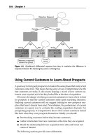
Another partitioning scheme, the DataSphere or DS, scales well with the
number of attributes and is sufficiently general. The number of classes in the
partition increases only linearly with the number of variables. The partitioning method consists of dividing the data into depth layers around the center
(like the layers of an onion) and superimposing directional pyramids to
capture the axis (attribute) related information. Every layer-pyramid combi-


12

exploratory data mining and data cleaning
DataSphere Partition in 2-D

Y+
a
a
a

a

X-

X+

YDepth quantile layers enclosing mass a;
Four pyramids in 2-D, Y+, Y-, X+, X-.
Figure 1.2: A DS partition in 2-D: Depth layers, directional puramids.

nation represents a class in the DS partition (see Figure 1.2). All the points
within a class are summarized using aggregates (EDM summaries) that can be
combined easily (sums, sum of products, counts). A detailed discussion is in
Section 3.4.
Two major uses of partition based summaries computed during EDM are
(a) to isolate data glitches and (b) to guide the choice of models for further
analyses. Fitting simple nonparametric models within each class of the partition and observing the changes from class to class can lead to an understanding of the nonlinear interactions between attributes. For example, fitting simple
survival functions within each class of a partition of the covariates can help us
to choose the appropriate proportional hazards model in a survival analysis
study. In some cases, such piecewise models can even function as approximations to more sophisticated models.

1.7 END-TO-END DATA QUALITY (DQ)
As noted earlier, data cleaning is an integral part of analysis. In fact,
DATA + ANALYSIS = RESULTS,
so that the effects of bad data and bad analysis are inseparable. The most

sophisticated analyses cannot wring intelligence out of bad data. Even worse,
if an analyst is unaware of data glitches, misleading results can be used to make
important decisions leading to lost credibility (wrong projections), lost revenues (billing errors), irate customers (billed twice) and sometimes fatalities
(incorrect computation of flight paths). Finding data glitches, publicizing them