Partially linear models
Bạn đang xem bản rút gọn của tài liệu. Xem và tải ngay bản đầy đủ của tài liệu tại đây (1.57 MB, 213 trang )
PARTIALLY LINEAR MODELS
Wolfgang H¨ardle
¨
Institut f¨
ur Statistik und Okonometrie
Humboldt-Universit¨at zu Berlin
D-10178 Berlin, Germany
Hua Liang
Department of Statistics
Texas A&M University
College Station
TX 77843-3143, USA
and
¨
Institut f¨
ur Statistik und Okonometrie
Humboldt-Universit¨at zu Berlin
D-10178 Berlin, Germany
Jiti Gao
School of Mathematical Sciences
Queensland University of Technology
Brisbane QLD 4001, Australia
and
Department of Mathematics and Statistics
The University of Western Australia
Perth WA 6907, Australia
ii
In the last ten years, there has been increasing interest and activity in the
general area of partially linear regression smoothing in statistics. Many methods
and techniques have been proposed and studied. This monograph hopes to bring
an up-to-date presentation of the state of the art of partially linear regression
techniques. The emphasis of this monograph is on methodologies rather than on
the theory, with a particular focus on applications of partially linear regression
techniques to various statistical problems. These problems include least squares
regression, asymptotically efficient estimation, bootstrap resampling, censored
data analysis, linear measurement error models, nonlinear measurement models,
nonlinear and nonparametric time series models.
We hope that this monograph will serve as a useful reference for theoretical
and applied statisticians and to graduate students and others who are interested
in the area of partially linear regression. While advanced mathematical ideas
have been valuable in some of the theoretical development, the methodological
power of partially linear regression can be demonstrated and discussed without
advanced mathematics.
This monograph can be divided into three parts: part one–Chapter 1 through
Chapter 4; part two–Chapter 5; and part three–Chapter 6. In the first part, we
discuss various estimators for partially linear regression models, establish theoretical results for the estimators, propose estimation procedures, and implement
the proposed estimation procedures through real and simulated examples.
The second part is of more theoretical interest. In this part, we construct
several adaptive and efficient estimates for the parametric component. We show
that the LS estimator of the parametric component can be modified to have both
Bahadur asymptotic efficiency and second order asymptotic efficiency.
In the third part, we consider partially linear time series models. First, we
propose a test procedure to determine whether a partially linear model can be
used to fit a given set of data. Asymptotic test criteria and power investigations
are presented. Second, we propose a Cross-Validation (CV) based criterion to
select the optimum linear subset from a partially linear regression and establish a CV selection criterion for the bandwidth involved in the nonparametric
v
vi
PREFACE
kernel estimation. The CV selection criterion can be applied to the case where
the observations fitted by the partially linear model (1.1.1) are independent and
identically distributed (i.i.d.). Due to this reason, we have not provided a separate chapter to discuss the selection problem for the i.i.d. case. Third, we provide
recent developments in nonparametric and semiparametric time series regression.
This work of the authors was supported partially by the Sonderforschungs¨
bereich 373 “Quantifikation und Simulation Okonomischer
Prozesse”. The second
author was also supported by the National Natural Science Foundation of China
and an Alexander von Humboldt Fellowship at the Humboldt University, while the
third author was also supported by the Australian Research Council. The second
and third authors would like to thank their teachers: Professors Raymond Carroll, Guijing Chen, Xiru Chen, Ping Cheng and Lincheng Zhao for their valuable
inspiration on the two authors’ research efforts. We would like to express our sincere thanks to our colleagues and collaborators for many helpful discussions and
stimulating collaborations, in particular, Vo Anh, Shengyan Hong, Enno Mammen, Howell Tong, Axel Werwatz and Rodney Wolff. For various ways in which
they helped us, we would like to thank Adrian Baddeley, Rong Chen, Anthony
Pettitt, Maxwell King, Michael Schimek, George Seber, Alastair Scott, Naisyin
Wang, Qiwei Yao, Lijian Yang and Lixing Zhu.
The authors are grateful to everyone who has encouraged and supported us
to finish this undertaking. Any remaining errors are ours.
Berlin, Germany
Texas, USA and Berlin, Germany
Perth and Brisbane, Australia
Wolfgang H¨ardle
Hua Liang
Jiti Gao
CONTENTS
PREFACE . . . . . . . . . . . . . . . . . . . . . . . . . . . . . . . . . . .
v
1 INTRODUCTION . . . . . . . . . . . . . . . . . . . . . . . . . . . .
1
1.1
Background, History and Practical Examples . . . . . . . . . . . .
1
1.2
The Least Squares Estimators . . . . . . . . . . . . . . . . . . . .
12
1.3
Assumptions and Remarks . . . . . . . . . . . . . . . . . . . . . .
14
1.4
The Scope of the Monograph . . . . . . . . . . . . . . . . . . . . .
16
1.5
The Structure of the Monograph . . . . . . . . . . . . . . . . . . .
17
2 ESTIMATION OF THE PARAMETRIC COMPONENT . . .
19
2.1
2.2
2.3
Estimation with Heteroscedastic Errors . . . . . . . . . . . . . . .
19
2.1.1
Introduction . . . . . . . . . . . . . . . . . . . . . . . . . .
19
2.1.2
Estimation of the Non-constant Variance Functions . . . .
22
2.1.3
Selection of Smoothing Parameters . . . . . . . . . . . . .
26
2.1.4
Simulation Comparisons . . . . . . . . . . . . . . . . . . .
27
2.1.5
Technical Details . . . . . . . . . . . . . . . . . . . . . . .
28
Estimation with Censored Data . . . . . . . . . . . . . . . . . . .
33
2.2.1
Introduction . . . . . . . . . . . . . . . . . . . . . . . . . .
33
2.2.2
Synthetic Data and Statement of the Main Results . . . .
33
2.2.3
Estimation of the Asymptotic Variance . . . . . . . . . . .
37
2.2.4
A Numerical Example . . . . . . . . . . . . . . . . . . . .
37
2.2.5
Technical Details . . . . . . . . . . . . . . . . . . . . . . .
38
Bootstrap Approximations . . . . . . . . . . . . . . . . . . . . . .
41
2.3.1
Introduction . . . . . . . . . . . . . . . . . . . . . . . . . .
41
2.3.2
Bootstrap Approximations . . . . . . . . . . . . . . . . . .
42
2.3.3
Numerical Results
43
. . . . . . . . . . . . . . . . . . . . . .
3 ESTIMATION OF THE NONPARAMETRIC COMPONENT 45
3.1
Introduction . . . . . . . . . . . . . . . . . . . . . . . . . . . . . .
45
viii
CONTENTS
3.2
Consistency Results . . . . . . . . . . . . . . . . . . . . . . . . . .
46
3.3
Asymptotic Normality . . . . . . . . . . . . . . . . . . . . . . . .
49
3.4
Simulated and Real Examples . . . . . . . . . . . . . . . . . . . .
50
3.5
Appendix . . . . . . . . . . . . . . . . . . . . . . . . . . . . . . .
53
4 ESTIMATION WITH MEASUREMENT ERRORS
. . . . . .
55
Linear Variables with Measurement Errors . . . . . . . . . . . . .
55
4.1.1
Introduction and Motivation . . . . . . . . . . . . . . . . .
55
4.1.2
Asymptotic Normality for the Parameters . . . . . . . . .
56
4.1.3
Asymptotic Results for the Nonparametric Part . . . . . .
58
4.1.4
Estimation of Error Variance
. . . . . . . . . . . . . . . .
58
4.1.5
Numerical Example . . . . . . . . . . . . . . . . . . . . . .
59
4.1.6
Discussions . . . . . . . . . . . . . . . . . . . . . . . . . .
61
4.1.7
Technical Details . . . . . . . . . . . . . . . . . . . . . . .
61
Nonlinear Variables with Measurement Errors . . . . . . . . . . .
65
4.2.1
Introduction . . . . . . . . . . . . . . . . . . . . . . . . . .
65
4.2.2
Construction of Estimators . . . . . . . . . . . . . . . . . .
66
4.2.3
Asymptotic Normality . . . . . . . . . . . . . . . . . . . .
67
4.2.4
Simulation Investigations . . . . . . . . . . . . . . . . . . .
68
4.2.5
Technical Details . . . . . . . . . . . . . . . . . . . . . . .
70
5 SOME RELATED THEORETIC TOPICS . . . . . . . . . . . . .
77
4.1
4.2
5.1
5.2
5.3
The Laws of the Iterated Logarithm . . . . . . . . . . . . . . . . .
77
5.1.1
Introduction . . . . . . . . . . . . . . . . . . . . . . . . . .
77
5.1.2
Preliminary Processes . . . . . . . . . . . . . . . . . . . .
78
5.1.3
Appendix . . . . . . . . . . . . . . . . . . . . . . . . . . .
79
The Berry-Esseen Bounds . . . . . . . . . . . . . . . . . . . . . .
82
5.2.1
Introduction and Results . . . . . . . . . . . . . . . . . . .
82
5.2.2
Basic Facts . . . . . . . . . . . . . . . . . . . . . . . . . .
83
5.2.3
Technical Details . . . . . . . . . . . . . . . . . . . . . . .
87
Asymptotically Efficient Estimation . . . . . . . . . . . . . . . . .
94
5.3.1
Motivation . . . . . . . . . . . . . . . . . . . . . . . . . . .
94
5.3.2
Construction of Asymptotically Efficient Estimators . . . .
94
5.3.3
Four Lemmas . . . . . . . . . . . . . . . . . . . . . . . . .
97
CONTENTS
5.3.4
5.4
5.5
5.6
ix
Appendix . . . . . . . . . . . . . . . . . . . . . . . . . . .
99
Bahadur Asymptotic Efficiency . . . . . . . . . . . . . . . . . . . 104
5.4.1
Definition . . . . . . . . . . . . . . . . . . . . . . . . . . . 104
5.4.2
Tail Probability . . . . . . . . . . . . . . . . . . . . . . . . 105
5.4.3
Technical Details . . . . . . . . . . . . . . . . . . . . . . . 106
Second Order Asymptotic Efficiency . . . . . . . . . . . . . . . . . 111
5.5.1
Asymptotic Efficiency . . . . . . . . . . . . . . . . . . . . 111
5.5.2
Asymptotic Distribution Bounds . . . . . . . . . . . . . . 113
5.5.3
Construction of 2nd Order Asymptotic Efficient Estimator 117
Estimation of the Error Distribution . . . . . . . . . . . . . . . . 119
5.6.1
Introduction . . . . . . . . . . . . . . . . . . . . . . . . . . 119
5.6.2
Consistency Results . . . . . . . . . . . . . . . . . . . . . . 120
5.6.3
Convergence Rates . . . . . . . . . . . . . . . . . . . . . . 124
5.6.4
Asymptotic Normality and LIL . . . . . . . . . . . . . . . 125
6 PARTIALLY LINEAR TIME SERIES MODELS . . . . . . . . 127
6.1
Introduction . . . . . . . . . . . . . . . . . . . . . . . . . . . . . . 127
6.2
Adaptive Parametric and Nonparametric Tests . . . . . . . . . . . 127
6.3
6.4
6.2.1
Asymptotic Distributions of Test Statistics . . . . . . . . . 127
6.2.2
Power Investigations of the Test Statistics . . . . . . . . . 131
Optimum Linear Subset Selection . . . . . . . . . . . . . . . . . . 136
6.3.1
A Consistent CV Criterion . . . . . . . . . . . . . . . . . . 136
6.3.2
Simulated and Real Examples . . . . . . . . . . . . . . . . 139
Optimum Bandwidth Selection . . . . . . . . . . . . . . . . . . . 144
6.4.1
Asymptotic Theory . . . . . . . . . . . . . . . . . . . . . . 144
6.4.2
Computational Aspects . . . . . . . . . . . . . . . . . . . . 150
6.5
Other Related Developments . . . . . . . . . . . . . . . . . . . . . 156
6.6
The Assumptions and the Proofs of Theorems . . . . . . . . . . . 157
6.6.1
Mathematical Assumptions . . . . . . . . . . . . . . . . . 157
6.6.2
Technical Details . . . . . . . . . . . . . . . . . . . . . . . 160
APPENDIX: BASIC LEMMAS . . . . . . . . . . . . . . . . . . . . . 183
REFERENCES . . . . . . . . . . . . . . . . . . . . . . . . . . . . . . . . 187
x
CONTENTS
AUTHOR INDEX . . . . . . . . . . . . . . . . . . . . . . . . . . . . . . 199
SUBJECT INDEX . . . . . . . . . . . . . . . . . . . . . . . . . . . . . 203
SYMBOLS AND NOTATION . . . . . . . . . . . . . . . . . . . . . . 205
1
INTRODUCTION
1.1 Background, History and Practical Examples
A partially linear regression model of the form is defined by
Yi = XiT β + g(Ti ) + εi , i = 1, . . . , n
(1.1.1)
where Xi = (xi1 , . . . , xip )T and Ti = (ti1 , . . . , tid )T are vectors of explanatory variables, (Xi , Ti ) are either independent and identically distributed (i.i.d.) random
design points or fixed design points. β = (β1 , . . . , βp )T is a vector of unknown parameters, g is an unknown function from IRd to IR1 , and ε1 , . . . , εn are independent
random errors with mean zero and finite variances σi2 = Eε2i .
Partially linear models have many applications. Engle, Granger, Rice and
Weiss (1986) were among the first to consider the partially linear model
(1.1.1). They analyzed the relationship between temperature and electricity usage.
We first mention several examples from the existing literature. Most of the
examples are concerned with practical problems involving partially linear models.
Example 1.1.1 Engle, Granger, Rice and Weiss (1986) used data based on the
monthly electricity sales yi for four cities, the monthly price of electricity x1 ,
income x2 , and average daily temperature t. They modeled the electricity demand
y as the sum of a smooth function g of monthly temperature t, and a linear
function of x1 and x2 , as well as with 11 monthly dummy variables x3 , . . . , x13 .
That is, their model was
13
y =
βj xj + g(t)
j=1
= X T β + g(t)
where g is a smooth function.
In Figure 1.1, the nonparametric estimates of the weather-sensitive load for
St. Louis is given by the solid curve and two sets of parametric estimates are
given by the dashed curves.
2
1. INTRODUCTION
Temperature response function for St. Louis. The nonparametric estimate is given by the solid curve, and the parametric estimates by the dashed
curves. From Engle, Granger, Rice and Weiss (1986), with permission from the
Journal of the American Statistical Association.
FIGURE 1.1.
Example 1.1.2 Speckman (1988) gave an application of the partially linear model
to a mouthwash experiment. A control group (X = 0) used only a water rinse for
mouthwash, and an experimental group (X = 1) used a common brand of analgesic. Figure 1.2 shows the raw data and the partially kernel regression estimates
for this data set.
Example 1.1.3 Schmalensee and Stoker (1999) used the partially linear model
to analyze household gasoline consumption in the United States. They summarized
the modelling framework as
LTGALS = G(LY, LAGE) + β1 LDRVRS + β2 LSIZE + β3T Residence
+β4T Region + β5 Lifecycle + ε
where LTGALS is log gallons, LY and LAGE denote log(income) and log(age)
respectively, LDRVRS is log(numbers of drive), LSIZE is log(household size), and
E(ε|predictor variables) = 0.
1. INTRODUCTION
3
Raw data partially linear regression estimates for mouthwash data.
The predictor variable is T = baseline SBI, the response is Y = SBI index after
three weeks. The SBI index is a measurement indicating gum shrinkage. From
Speckman (1988), with the permission from the Royal Statistical Society.
FIGURE 1.2.
Figures 1.3 and 1.4 depicts log-income profiles for different ages and logage profiles for different incomes. The income structure is quite clear from 1.3.
Similarly, 1.4 shows a clear age structure of household gasoline demand.
Example 1.1.4 Green and Silverman (1994) provided an example of the use of
partially linear models, and compared their results with a classical approach employing blocking. They considered the data, primarily discussed by Daniel and
Wood (1980), drawn from a marketing price-volume study carried out in the
petroleum distribution industry.
The response variable Y is the log volume of sales of gasoline, and the two
main explanatory variables of interest are x1 , the price in cents per gallon of gasoline, and x2 , the differential price to competition. The nonparametric component
t represents the day of the year.
Their analysis is displayed in Figure 1.5 1 . Three separate plots against t are
1
The postscript files of Figures 1.5-1.7 are provided by Professor Silverman.
4
1. INTRODUCTION
Income structure, 1991. From Schmalensee and Stoker (1999), with
the permission from the Journal of Econometrica.
FIGURE 1.3.
shown. Upper plot: parametric component of the fit; middle plot: dependence on
nonparametric component; lower plot: residuals. All three plots are drown to the
same vertical scale, but the upper two plots are displaced upwards.
Example 1.1.5 Dinse and Lagakos (1983) reported on a logistic analysis of some
bioassay data from a US National Toxicology Program study of flame retardants.
Data on male and female rates exposed to various doses of a polybrominated
biphenyl mixture known as Firemaster FF-1 consist of a binary response variable, Y , indicating presence or absence of a particular nonlethal lesion, bile duct
hyperplasia, at each animal’s death. There are four explanatory variables: log dose,
x1 , initial weight, x2 , cage position (height above the floor), x3 , and age at death,
t. Our choice of this notation reflects the fact that Dinse and Lagakos commented
on various possible treatments of this fourth variable. As alternatives to the use
of step functions based on age intervals, they considered both a straightforward
linear dependence on t, and higher order polynomials. In all cases, they fitted
a conventional logistic regression model, the GLM data from male and female
rats separate in the final analysis, having observed interactions with gender in an
1. INTRODUCTION
5
Age structure, 1991. From Schmalensee and Stoker (1999), with the
permission from the Journal of Econometrica.
FIGURE 1.4.
initial examination of the data.
Green and Yandell (1985) treated this as a semiparametric GLM regression
problem, regarding x1 , x2 and x3 as linear variables, and t the nonlinear variable. Decompositions of the fitted linear predictors for the male and female rats
are shown in Figures 1.6 and 1.7, based on the Dinse and Lagakos data sets,
consisting of 207 and 112 animals respectively.
Furthermore, let us now cite two examples of partially linear models that may
typically occur in microeconomics, constructed by Tripathi (1997). In these two
examples, we are interested in estimating the parametric component when we
only know that the unknown function belongs to a set of appropriate functions.
Example 1.1.6 A firm produces two different goods with production functions
F1 and F2 . That is, y1 = F1 (x) and y2 = F2 (z), with (x × z) ∈ Rn × Rm . The firm
1. INTRODUCTION
0.3
0.2
0.0
0.1
Decomposition
0.4
0.5
6
50
100
150
200
Time
Partially linear decomposition of the marketing data. Results taken
from Green and Silverman (1994) with permission of Chapman & Hall.
FIGURE 1.5.
maximizes total profits p1 y1 − w1T x = p2 y2 − w2T z. The maximized profit can be
written as π1 (u) + π2 (v), where u = (p1 , w1 ) and v = (p2 , w2 ). Now suppose that
the econometrician has sufficient information about the first good to parameterize
the first profit function as π1 (u) = uT θ0 . Then the observed profit is πi = uTi θ0 +
π2 (vi ) + εi , where π2 is monotone, convex, linearly homogeneous and continuous
in its arguments.
Example 1.1.7 Again, suppose we have n similar but geographically dispersed
firms with the same profit function. This could happen if, for instance, these firms
had access to similar technologies. Now suppose that the observed profit depends
not only upon the price vector, but also on a linear index of exogenous variables.
That is, πi = xTi θ0 +π ∗ (p1 , . . . , pk )+εi , where the profit function π ∗ is continuous,
monotone, convex, and homogeneous of degree one in its arguments.
Partially linear models are semiparametric models since they contain
both parametric and nonparametric components. It allows easier interpretation
of the effect of each variable and may be preferred to a completely nonparametric
1. INTRODUCTION
7
•
•
• •
•
4
+
+ ++ ++++ + +
+
+++
+
+
+
++ + + +++
+
++ ++++
+++ +++++++++
+
+
++++ +
2
Decomposition
6
•
•
•
•
•
• • • • • • • • •• • • • •• • • •• ••• • • •• • • • • • • ••• •
• •
• • •• • • •• •• • •• • •• •• •• • • • • •• • • • ••• ••
• •• •
•
•
•
•
•
•
•
•
•
•
•
•
•
•
•
•
•
• • • • • • • • • ••• • • • • • • • • • • • • • •• • • • •
•
• • • •• •
••• • • • •
•
•
+
0
+
+
+
40
+
+
+
60
+++++ ++++++
+++++++++++++++
++++ +++
++++ ++++++++++ ++++++++++++++++ +
+
+
+
+
+
+
+
+
+
+ + ++ +
+ + +
+
80
100
120
Time
Semiparametric logistic regression analysis for male data. Results
taken from Green and Silverman (1994) with permission of Chapman & Hall.
FIGURE 1.6.
regression because of the well-known “curse of dimensionality”. The parametric
√
components can be estimated at the rate of n, while the estimation precision of
the nonparametric function decreases rapidly as the the dimension of the nonlinear variable increases. Moreover, the partially linear models are more flexible than
the standard linear models, since they combine both parametric and nonparametric components when it is believed that the response depends on some variables
in linear relationship but is nonlinearly related to other particular independent
variables.
Following the work of Engle, Granger, Rice and Weiss (1986), much attention has been directed to estimating (1.1.1). See, for example, Heckman (1986),
Rice (1986), Chen (1988), Robinson (1988), Speckman (1988), Hong (1991), Gao
(1992), Liang (1992), Gao and Zhao (1993), Schick (1996a,b) and Bhattacharya
and Zhao (1993) and the references therein. For instance, Robinson (1988) constructed a feasible least squares estimator of β based on estimating the nonparametric component by a Nadaraya-Waston kernel estimator. Under some regularity
conditions, he deduced the asymptotic distribution of the estimate.
1. INTRODUCTION
20
8
• •
•
•
•
15
•
•
•
•
•
•
•
•
•
•
•
•
• •
•
•
•• • •
• • • •• ••
•
• • ••
• • • • •• ••
••
• • •• ••
•• • ••
• • • • •• ••
•
•
•
• ••
• • •
•
10
5
Decomposition
•
• •
•
•
•
•
•
•
• •••
• • •
• •• •
• • • •
•
•
•
+
+
0
+
+
+
40
+
+
60
+
+
+
++ +++ +++
+
80
+
+
+
+
+
+ +
+ +++ + +++++ + ++++ +++++++
+ ++++ ++++ ++++ + ++++++ ++ ++ +
+
+
100
120
Time
Semiparametric logistic regression analysis for female data. Results
taken from Green and Silverman (1994) with permission of Chapman & Hall.
FIGURE 1.7.
Speckman (1988) argued that the nonparametric component can be characterized by Wγ, where W is a (n × q)−matrix of full rank, γ is an additional
unknown parameter and q is unknown. The partially linear model (1.1.1)
can be rewritten in a matrix form
Y = Xβ + Wγ + ε.
(1.1.2)
The estimator of β based on (1.1.2) is
β = {XT (F − PW )X)}−1 {XT (F − PW )Y)}
(1.1.3)
where PW = W(W T W)−1 W T is a projection matrix. Under some suitable conditions, Speckman (1988) studied the asymptotic behavior of this estimator. This
estimator is asymptotically unbiased because β is calculated after removing the
influence of T from both the X and Y . (See (3.3a) and (3.3b) of Speckman (1988)
and his kernel estimator thereafter). Green, Jennison and Seheult (1985) proposed
to replace W in (1.1.3) by a smoothing operator for estimating β as follows:
βGJS = {XT (F − Wh )X)}−1 {XT (F − Wh )Y)}.
(1.1.4)
1. INTRODUCTION
9
Following Green, Jennison and Seheult (1985), Gao (1992) systematically
studied asymptotic behaviors of the least squares estimator given by (1.1.3) for
the case of non-random design points.
Engle, Granger, Rice and Weiss (1986), Heckman (1986), Rice (1986), Whaba
(1990), Green and Silverman (1994) and Eubank, Kambour, Kim, Klipple, Reese
and Schimek (1998) used the spline smoothing technique and defined the penalized estimators of β and g as the solution of
1 n
argminβ,g
{Yi − XiT β − g(Ti )}2 + λ
n i=1
{g (u)}2 du
(1.1.5)
where λ is a penalty parameter (see Whaba (1990)). The above estimators are
asymptotically biased (Rice, 1986, Schimek, 1997). Schimek (1999) demonstrated
in a simulation study that this bias is negligible apart from small sample sizes
(e.g. n = 50), even when the parametric and nonparametric components are
correlated.
The original motivation for Speckman’s algorithm was a result of Rice (1986),
who showed that within a certain asymptotic framework, the penalized least
squares (PLS) estimate of β could be susceptible to biases of the kind that are inevitable when estimating a curve. Heckman (1986) only considered the case where
Xi and Ti are independent and constructed an asymptotically normal estimator
for β. Indeed, Heckman (1986) proved that the PLS estimator of β is consistent
at parametric rates if small values of the smoothing parameter are used. Hamilton and Truong (1997) used local linear regression in partially linear models
and established the asymptotic distributions of the estimators of the parametric and nonparametric components. More general theoretical results along with
these lines are provided by Cuzick (1992a), who considered the case where the
density of ε is known. See also Cuzick (1992b) for an extension to the case where
the density function of ε is unknown. Liang (1992) systematically studied the
Bahadur efficiency and the second order asymptotic efficiency for a numbers of cases. More recently, Golubev and H¨ardle (1997) derived the upper and
lower bounds for the second minimax order risk and showed that the second
order minimax estimator is a penalized maximum likelihood estimator. Similarly, Mammen and van de Geer (1997) applied the theory of empirical processes
to derive the asymptotic properties of a penalized quasi likelihood estimator,
which generalizes the piecewise polynomial-based estimator of Chen (1988).
10
1. INTRODUCTION
In the case of heteroscedasticity, Schick (1996b) constructed root-n consistent weighted least squares estimates and proposed an optimal weight function
for the case where the variance function is known up to a multiplicative constant.
More recently, Liang and H¨ardle (1997) further studied this issue for more general
variance functions.
Severini and Staniswalis (1994) and H¨ardle, Mammen and M¨
uller (1998) studied a generalization of (1.1.1), which corresponds to
E(Y |X, T ) = H{X T β + g(T )}
(1.1.6)
where H (called link function) is a known function, and β and g are the same as
in (1.1.1). To estimate β and g, Severini and Staniswalis (1994) introduced the
quasi-likelihood estimation method, which has properties similar to those of the
likelihood function, but requires only specification of the second-moment properties of Y rather than the entire distribution. Based on the approach of Severini
and Staniswalis, H¨ardle, Mammen and M¨
uller (1998) considered the problem of
testing the linearity of g. Their test indicates whether nonlinear shapes observed
in nonparametric fits of g are significant. Under the linear case, the test statistic
is shown to be asymptotically normal. In some sense, their test complements the
work of Severini and Staniswalis (1994). The practical performance of the tests is
shown in applications to data on East-West German migration and credit scoring. Related discussions can also be found in Mammen and van de Geer (1997)
and Carroll, Fan, Gijbels and Wand (1997).
Example 1.1.8 Consider a model on East–West German migration in 1991
GSOEP (1991)data from the German Socio-Economic Panel for the state Mecklenburg-Vorpommern, a land of the Federal State of Germany. The dependent
variable is binary with Y = 1 (intention to move) or Y = 0 (stay). Let X denote
some socioeconomic factors such as age, sex, friends in west, city size and unemployment, T do household income. Figure 1.8 shows a fit of the function g in the
semiparametric model (1.1.6). It is clearly nonlinear and shows a saturation in
the intention to migrate for higher income households. The question is, of course,
whether the observed nonlinearity is significant.
Example 1.1.9 M¨
uller and R¨
onz (2000) discuss credit scoring methods which
aim to assess credit worthiness of potential borrowers to keep the risk of credit
1. INTRODUCTION
11
0.0
-0.2
-0.6
-0.4
m(hosehold income)
0.2
0.4
Household income -> Migration
0.5
1.0
1.5
2.0
2.5
household income
3.0
(*10 3 )
3.5
4.0
The influence of household income (function g(t)) on migration intention. Sample from Mecklenburg–Vorpommern, n = 402.
FIGURE 1.8.
loss low and to minimize the costs of failure over risk groups. One of the classical
parametric approaches, logit regression, assumes that the probability of belonging
to the group of “bad” clients is given by P (Y = 1) = F (β T X), with Y = 1 indicating a “bad” client and X denoting the vector of explanatory variables, which
include eight continuous and thirteen categorical variables. X2 to X9 are the continuous variables. All of them have (left) skewed distributions. The variables X6
to X9 in particular have one realization which covers the majority of observations.
X10 to X24 are the categorical variables. Six of them are dichotomous. The others
have 3 to 11 categories which are not ordered. Hence, these variables have been
categorized into dummies for the estimation and validation.
The authors consider a special case of the generalized partially linear model
E(Y |X, T ) = G{β T X + g(T )} which allows to model the influence of a part T of
the explanatory variables in a nonparametric way. The model they study is
P (Y = 1) = F g(x5 ) +
24
j=2,j=5
βj xj
where a possible constant is contained in the function g(·). This model is estimated
by semiparametric maximum–likelihood, a combination of ordinary and smoothed
maximum–likelihood. Figure 1.9 compares the performance of the parametric logit
fit and the semiparametric logit fit obtained by including X5 in a nonparametric
way. Their analysis indicated that this generalized partially linear model improves
12
1. INTRODUCTION
the previous performance. The detailed discussion can be found in M¨
uller and
R¨
onz (2000).
0
P(S
1
Performance X5
0
0.5
P(S
1
Performance curves, parametric logit (black dashed) and semiparametric logit (thick grey) with variable X5 included nonparametrically. Results
taken from M¨
uller and R¨onz (2000).
FIGURE 1.9.
1.2 The Least Squares Estimators
If the nonparametric component of the partially linear model is assumed to be
known, then LS theory may be applied. In practice, the nonparametric component g, regarded as a nuisance parameter, has to be estimated through smoothing
methods. Here we are mainly concerned with the nonparametric regression estimation. For technical convenience, we focus only on the case of T ∈ [0, 1] in
Chapters 2-5. In Chapter 6, we extend model (1.1.1) to the multi-dimensional
time series case. Therefore some corresponding results for the multidimensional
independent case follow immediately, see for example, Sections 6.2 and 6.3.
For identifiability, we assume that the pair (β, g) of (1.1.1) satisfies
1 n
1 n
T
2
E{Yi − Xi β − g(Ti )} = min
E{Yi − XiT α − f (Ti )}2 .
(α,f ) n
n i=1
i=1
(1.2.1)
1. INTRODUCTION
13
This implies that if XiT β1 + g1 (Ti ) = XiT β2 + g2 (Ti ) for all 1 ≤ i ≤ n, then β1 = β2
and g1 = g2 simultaneously. We will justify this separately for the random design
case and the fixed design case.
For the random design case, if we assume that E[Yi |(Xi , Ti )] = XiT β1 +
g1 (Ti ) = XiT β2 + g2 (Ti ) for all 1 ≤ i ≤ n, then it follows from E{Yi − XiT β1 −
g1 (Ti )}2 = E{Yi −XiT β2 −g2 (Ti )}2 +(β1 −β2 )T E{(Xi −E[Xi |Ti ])(Xi −E[Xi |Ti ])T }
(β1 − β2 ) that we have β1 = β2 due to the fact that the matrix E{(Xi −
E[Xi |Ti ])(Xi − E[Xi |Ti ])T } is positive definite assumed in Assumption 1.3.1(i)
below. Thus g1 = g2 follows from the fact gj (Ti ) = E[Yi |Ti ] − E[XiT βj |Ti ] for all
1 ≤ i ≤ n and j = 1, 2.
For the fixed design case, we can justify the identifiability using several different methods. We here provide one of them. Suppose that g of (1.1.1) can be
parameterized as G = {g(T1 ), . . . , g(Tn )}T = W γ used in (1.2.2), where γ is a
vector of unknown parameters.
Then submitting G = W γ into (1.2.1), we have the normal equations
X T Xβ = X T (Y − W γ) and W γ = P (Y − Xβ),
where P = W (W T W )−1 W T , X T = (X1 , . . . , Xn ) and Y T = (Y1 , . . . , Yn ).
Similarly, if we assume that E[Yi ] = XiT β1 + g1 (Ti ) = XiT β2 + g2 (Ti ) for all
1 ≤ i ≤ n, then it follows from Assumption 1.3.1(ii) below and the fact that
1/nE{(Y − Xβ1 − W γ1 )T (Y − Xβ1 − W γ1 )} = 1/nE{(Y − Xβ2 − W γ2 )T (Y −
Xβ2 − W γ2 )} + 1/n(β1 − β2 )T X T (I − P )X(β1 − β2 ) that we have β1 = β2 and
g1 = g2 simultaneously.
Assume that {(Xi , Ti , Yi ); i = 1, . . . , n.} satisfies model (1.1.1). Let ωni (t){=
ωni (t; T1 , . . . , Tn )} be positive weight functions depending on t and the design
points T1 , . . . , Tn . For every given β, we define an estimator of g(·) by
n
ωnj (t)(Yi − XiT β).
gn (t; β) =
i=1
We often drop the β for convenience. Replacing g(Ti ) by gn (Ti ) in model (1.1.1)
and using the LS criterion, we obtain the least squares estimator of β:
βLS = (XT X)−1 XT Y,
(1.2.2)
which is just the estimator βGJS in (1.1.4) with a different smoothing operator.
14
1. INTRODUCTION
The nonparametric estimator of g(t) is then defined as follows:
n
ωni (t)(Yi − XiT βLS ).
gn (t) =
(1.2.3)
i=1
where XT = (X1 , . . . , Xn ) with Xj = Xj −
with Yj = Yj −
n
i=1
n
i=1
ωni (Tj )Xi and YT = (Y1 , . . . , Yn )
ωni (Tj )Yi . Due to Lemma A.2 below, we have as n → ∞
n−1 (XT X) → Σ, where Σ is a positive matrix. Thus, we assume that n(XT X)−1
exists for large enough n throughout this monograph.
When ε1 , . . . , εn are identically distributed, we denote their distribution function by ϕ(·) and the variance by σ 2 , and define the estimator of σ 2 by
σn2 =
1 n
(Yi − XiT βLS )2
n i=1
(1.2.4)
In this monograph, most of the estimation procedures are based on the estimators
(1.2.2), (1.2.3) and (1.2.4).
1.3 Assumptions and Remarks
This monograph considers the two cases: the fixed design and the i.i.d. random
design. When considering the random case, denote
hj (Ti ) = E(xij |Ti ) and uij = xij − E(xij |Ti ).
Assumption 1.3.1 i) sup0≤t≤1 E( X1 3 |T = t) < ∞ and Σ = Cov{X1 −
E(X1 |T1 )} is a positive definite matrix. The random errors εi are independent
of (Xi , Ti ).
ii) When (Xi , Ti ) are fixed design points, there exist continuous functions
hj (·) defined on [0, 1] such that each component of Xi satisfies
xij = hj (Ti ) + uij 1 ≤ i ≤ n, 1 ≤ j ≤ p
(1.3.1)
where {uij } is a sequence of real numbers satisfying
1 n
ui uTi = Σ
n→∞ n
i=1
lim
(1.3.2)
and for m = 1, . . . , p,
lim sup
n→∞
1
max
an 1≤k≤n
k
uji m < ∞
(1.3.3)
i=1
for all permutations (j1 , . . . , jn ) of (1, 2, . . . , n), where ui = (ui1 , . . . , uip )T , an =
n1/2 log n, and Σ is a positive definite matrix.
1. INTRODUCTION
15
Throughout the monograph, we apply Assumption 1.3.1 i) to the case of
random design points and Assumption 1.3.1 ii) to the case where (Xi , Ti ) are
fixed design points. Assumption 1.3.1 i) is a reasonable condition for the
random design case, while Assumption 1.3.1 ii) generalizes the corresponding
conditions of Heckman (1986) and Rice (1986), and simplifies the conditions of
Speckman (1988). See also Remark 2.1 (i) of Gao and Liang (1997).
Assumption 1.3.2 The first two derivatives of g(·) and hj (·) are Lipschitz
continuous of order one.
Assumption 1.3.3 When (Xi , Ti ) are fixed design points, the positive weight
functions ωni (·) satisfy
n
(i)
max
1≤i≤n
ωni (Tj ) = O(1),
j=1
n
max
1≤j≤n
(ii)
ωni (Tj ) = O(1),
i=1
max ωni (Tj ) = O(bn ),
1≤i,j≤n
n
ωnj (Ti )I(|Ti − Tj | > cn ) = O(cn ),
(iii) max
1≤i≤n
j=1
where bn and cn are two sequences satisfying lim sup nb2n log4 n < ∞, lim
inf nc2n >
n→∞
n→∞
0, lim sup nc4n log n < ∞ and lim sup nb2n c2n < ∞. When (Xi , Ti ) are i.i.d. random
n→∞
n→∞
design points, (i), (ii) and (iii) hold with probability one.
Remark 1.3.1 There are many weight functions satisfying Assumption 1.3.3.
For examples,
(1)
Wni (t) =
1
hn
Si
K
Si−1
t−s
t − Ti
(2)
ds, Wni (t) = K
Hn
Hn
n
K
j=1
t − Tj
,
Hn
where Si = 12 (T(i) + T(i−1) ), i = 1, · · · , n − 1, S0 = 0, Sn = 1, and T(i) are the
order statistics of {Ti }. K(·) is a kernel function satisfying certain conditions,
and Hn is a positive number sequence. Here Hn = hn or rn , hn is a bandwidth
parameter, and rn = rn (t, T1 , · · · , Tn ) is the distance from t to the kn −th nearest
neighbor among the Ti s, and where kn is an integer sequence.
(1)
(2)
We can justify that both Wni (t) and Wni (t) satisfy Assumption 1.3.3. The
details of the justification are very lengthy and omitted. We also want to point
16
1. INTRODUCTION
(1)
(2)
out that when ωni is either Wni or Wni , Assumption 1.3.3 holds automatically
with Hn = λn−1/5 for some 0 < λ < ∞. This is the same as the result established
by Speckman (1988) (see Theorem 2 with ν = 2), who pointed out that the usual
n−1/5 rate for the bandwidth is fast enough to establish that the LS estimate βLS
√
of β is n-consistent. Sections 2.1.3 and 6.4 will discuss some practical selections
for the bandwidth.
Remark 1.3.2 Throughout this monograph, we are mostly using Assumption
1.3.1 ii) and 1.3.3 for the fixed design case. As a matter of fact, we can replace
Assumption 1.3.1 ii) and 1.3.3 by the following corresponding conditions.
Assumption 1.3.1 ii)’ When (Xi , Ti ) are the fixed design points, equations
(1.3.1) and (1.3.2) hold.
Assumption 1.3.3’ When (Xi , Ti ) are fixed design points, Assumption 1.3.3
(i)-(iii) holds. In addition, the weight functions ωni satisfy
n
(iv) max
1≤i≤n
ωnj (Ti )ujl = O(dn ),
j=1
(v)
1 n
fj ujl = O(dn ),
n j=1
(vi)
1 n
n j=1
n
ωnk (Tj )uks ujl = O(dn )
k=1
for all 1 ≤ l, s ≤ p, where dn is a sequence of real numbers satisfying lim sup nd4n
n→∞
log n < ∞, fj = f (Tj ) −
n
k=1
ωnk (Tj )f (Tk ) for f = g or hj defined in (1.3.1).
Obviously, the three conditions (iv), (v) and (vi) follows from (1.3.3) and
Abel’s inequality.
(2)
When the weight functions ωni are chosen as Wni defined in Remark 1.3.1,
Assumptions 1.3.1 ii)’ and 1.3.3’ are almost the same as Assumptions (a)-(f ) of
Speckman (1988). As mentioned above, however, we prefer to use Assumptions
1.3.1 ii) and 1.3.3 for the fixed design case throughout this monograph.
Under the above assumptions, we provide bounds for hj (Ti ) −
hj (Tk ) and g(Ti ) −
n
k=1
n
k=1
ωnk (Ti )
ωnk (Ti )g(Tk ) in the appendix.
1.4 The Scope of the Monograph
The main objectives of this monograph are: (i) To present a number of theoretical results for the estimators of both parametric and nonparametric components,
1. INTRODUCTION
17
and (ii) To illustrate the proposed estimation and testing procedures by several
simulated and true data sets using XploRe-The Interactive Statistical Computing Environment (see H¨ardle, Klinke and M¨
uller, 1999), available on website:
.
In addition, we generalize the existing approaches for homoscedasticity to
heteroscedastic models, introduce and study partially linear errors-in-variables
models, and discuss partially linear time series models.
1.5 The Structure of the Monograph
The monograph is organized as follows: Chapter 2 considers a simple partially
linear model. An estimation procedure for the parametric component of the partially linear model is established based on the nonparametric weight sum. Section
2.1 mainly provides asymptotic theory and an estimation procedure for the parametric component with heteroscedastic errors. In this section, the least squares
estimator βLS of (1.2.2) is modified to the weighted least squares estimator βW LS .
For constructing βW LS , we employ the split-sample techniques. The asymptotic normality of βW LS is then derived. Three different variance functions are
discussed and estimated. The selection of smoothing parameters involved in the
nonparametric weight sum is also discussed in Subsection 2.1.3. Simulation comparison is also implemented in Subsection 2.1.4. A modified estimation procedure
for the case of censored data is given in Section 2.2. Based on a modification of
the Kaplan-Meier estimator, synthetic data and an estimator of β are constructed. We then establish the asymptotic normality for the resulting estimator
of β. We also examine the behaviors of the finite sample through a simulated
example. Bootstrap approximations are given in Section 2.3.
Chapter 3 discusses the estimation of the nonparametric component without
the restriction of constant variance. Convergence and asymptotic normality of the
nonparametric estimate are given in Sections 3.2 and 3.3. The estimation methods
proposed in this chapter are illustrated through examples in Section 3.4, in which
the estimator (1.2.3) is applied to the analysis of the logarithm of the earnings
to labour market experience.
In Chapter 4, we consider both linear and nonlinear variables with measurement errors. An estimation procedure and asymptotic theory for the case where