CO2 Emissions energy consumption and economic grow

See discussions, stats, and author profiles for this publication at: />
CO2 emissions, energy consumption and economic growth in Association of
Southeast Asian Nations (ASEAN) countries: A cointegration approach
Article  in  Energy · June 2013
DOI: 10.1016/j.energy.2013.04.038

CITATIONS

READS

130

1,132

2 authors, including:
Behnaz Saboori
Islamic Azad University, South Tehran Branch
25 PUBLICATIONS   874 CITATIONS   
SEE PROFILE

Some of the authors of this publication are also working on these related projects:

Asia Pacific gas market View project

All content following this page was uploaded by Behnaz Saboori on 10 April 2018.

The user has requested enhancement of the downloaded file.


Energy 55 (2013) 813e822

Contents lists available at SciVerse ScienceDirect

Energy
journal homepage: www.elsevier.com/locate/energy

CO2 emissions, energy consumption and economic growth in
Association of Southeast Asian Nations (ASEAN) countries:
A cointegration approach
Behnaz Saboori*, Jamalludin Sulaiman
Economic Programme, School of Social Sciences, Universiti Sains Malaysia, 11800 USM Penang, Malaysia

a r t i c l e i n f o

a b s t r a c t

Article history:
Received 28 November 2012
Received in revised form
15 February 2013
Accepted 14 April 2013
Available online 20 May 2013

This study examines the cointegration and causal relationship between economic growth, carbon dioxide
(CO2) emissions and energy consumption in selected Association of Southeast Asian Nations (ASEAN)
countries for the period 1971e2009. The recently developed Autoregressive Distributed Lag (ARDL)
methodology and Granger causality test based on Vector Error-Correction Model (VECM) were used to
conduct the analysis. There was cointegration relationship between variables in all the countries under
the study with statistically significant positive relationship between carbon emissions and energy consumption in both the short and long-run. The long-run elasticities of energy consumption with respect to
carbon emissions are higher than the short-run elasticities. This implies that carbon emissions level is
found to increase in respect to energy consumption over time in the selected ASEAN countries. A significant non-linear relationship between carbon emissions and economic growth was supported in

Singapore and Thailand for the long-run which supports the Environmental Kuznets Curve (EKC) hypothesis. The Granger causality results suggested a bi-directional Granger causality between energy
consumption and CO2 emissions in all the five ASEAN countries. This implies that carbon emissions and
energy consumption are highly interrelated to each other. All the variables are found to be stable suggesting that all the estimated models are stable over the study period.
Ó 2013 Elsevier Ltd. All rights reserved.

Keywords:
Carbon dioxide emissions
Energy consumption
Economic growth

1. Introduction
The debate about the relationship between energy consumption
and economic development stems from the increasing effects of
energy on economic development. With growing concerns about
global warming or climate change, there is a pressure for nations to
consume a balanced level of energy that control the emissions to
the environment; but at the same time ensuring the country’s
sustainable economic growth.
Testing the relationship between economic growth and environmental pollution under the Environmental Kuznets Curve (EKC)
hypothesis forms the first group of related literatures. The EKC
hypothesis claims an inverted U-shaped relationship between
environmental pollution and income per capita. However related
empirical studies are inconclusive. Although Shafik and Bandyopadhyay [1], Seldon and Song [2], Unruh and Moomaw [3], Galeotti
and Lanza [4], Dinda and Coondoo [5] and Managi and Jena [6] have

* Corresponding author. Tel.: þ60 176168939.
E-mail address: (B. Saboori).
0360-5442/$ e see front matter Ó 2013 Elsevier Ltd. All rights reserved.
/>
found evidence supporting the existence of an EKC, many others

have found evidences against the hypothesis (see e.g. Refs. [7e12]).1
The second group of studies examined the relationship between
economic growth and energy consumption. Since the seminal
study by Kraft and Kraft [16], more literatures have emerged
examining the cointegration and causality relationship between
economic growth and energy consumption (see Refs. [17e20] for
recent studies).
Later due to the omitted variable biased embodied in the first
and second group of literatures, a third group was formed, which
tested the relationship between economic growth, energy consumption and pollution emissions in a multivariate framework.
They address the problem of omitted variable bias that may yield
spurious results for the EKC hypothesis and the nature of the
causality.
Some recent examples of studies for developed countries
include by Ang [21] for France, Soytas et al. [22] for the United

1
An extensive review of EKC literature is available in papers of Stern [13], Dinda
[14] and Kijima et al. [15].


814

B. Saboori, J. Sulaiman / Energy 55 (2013) 813e822
CO emissions per capita in logs

Energy consumption per capita in logs

11.5

10.0

11.0
9.6

10.5
10.0

9.2

9.5
9.0

8.8

8.5
8.0
1975

1980

1985

1990

1995

2000

2005

8.4
1975

1980

1985

1990

1995

2000

2005

GDP per capita in logs
11.2
10.8
10.4
10.0
9.6
9.2
8.8
1975

1980

1985

1990

1995

2000

2005

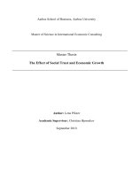
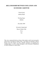
Fig. 1. Time series plots of real GDP per capita (constant US$), carbon emissions per capita (metric tons oil equivalent) and per capita energy consumption (kg of oil equivalent) in
log levels in the ASEAN countries.

States and Acaravci and Ozturk [23] for nineteen European countries. There are recent studies for developing countries such as Ang
[24] for Malaysia, Zhang and Cheng [25] for China, Ghosh [26] for
India, Lotfalipour et al. [27] for Iran, Menyah and Rufael [28] for
South Africa and Ozturk and Acaravci [29] for Turkey.2 However no
consensus finding has emerged from these studies. This makes the
recommendation of a unique policy across countries impossible at
this point in time.
For example, Ang [21] argues an inverted U-shaped relationship
between CO2 emissions and output for France thus suggesting the
evidence of EKC. He found a long-run relationship between output,
CO2 emissions and energy consumption with a causal relationship
from output to energy consumption and CO2 emissions in the longrun and from energy consumption to economic growth in the
short-run. Soytas et al. [22] found that income does not cause CO2
emissions in the United States in the long-run, but energy consumption does. Using Autoregressive Distributed Lag (ARDL)
bounds testing approach of cointegration for nineteen European
countries Acaravci and Ozturk [23] found a cointegration relationship between CO2 emissions, energy consumption and real income
for Denmark, Germany, Greece, Iceland, Italy, Portugal and
Switzerland. The EKC was satisfied just in the cases of Denmark and
Italy. Ang [24] and Zhang and Cheng [25] in the cases of Malaysia

and China respectively found a unidirectional Granger causality
running from GDP to energy consumption in long-run.
Ghosh [26] showed that there is a bi-directional causality between carbon emissions and economic growth in India and a unidirectional causality running from economic growth to energy
supply and energy supply to carbon emissions in the short-run.
Contrary to other studies, Menyah and Rufael [28] in a study for
South Africa found a unidirectional causality running from pollutant
emissions to economic growth and from energy consumption to

2
There are panel-based Granger causality studies of the CO2 emissions-economic
growth-energy consumption nexus such as Apergis and Payne [30] for Central
American countries, Apergis and Payne [31] for a panel of the Commonwealth of
Independent States, Lean and Smyth [32] for five members of ASEAN countries, Pao
and Tsai [33] for BRIC (Brazil, Russia, India and China) countries, Al-mulali and Binti
Che Sab [34] for Sub Saharan African countries and Bashiri Behmiri and Pires Manso
[35] for OECD countries.

economic growth and CO2 emissions. Similarly, Lotfalipour et al.
[27] found a unidirectional causality from energy consumption to
CO2 emissions for Iran. Ozturk and Acaravci [29] show that neither
carbon emissions per capita nor energy consumption per capita
influences real GDP (Gross Domestic Product) per capita in Turkey.
Luzzati and Orsini [36] investigated the relationship between absolute energy consumption and GDP per capita for 113 countries.
The results did not support an energy-EKC hypothesis for the world
as a single unit however, they found a positive monotonic relationship between carbon emissions and economic growth.
In 1967, the Association of Southeast Asian Nations (ASEAN) was
formed consisting of Indonesia, Malaysia, Philippines, Singapore
and Thailand. Since then membership has expanded to include
Brunei Darussalam, Vietnam, Laos, Myanmar and Cambodia making up what is today the ten member states of ASEAN. The region is
surrounded by major seas and gulfs such as the South China Sea,

the Andaman Sea and the gulf of Thailand. It has a total land area of
4.436 million square kilometers (3.3% of the world’s land area) and
a total population of 584 million (8.7% of the world population).
ASEAN is one of the fastest growing economic regions in the
world. Its economy has experienced a rapid GDP growth at an
average annual rate of 4.8 and 6.5 percent for 1994e1999 and
2000e2008 periods respectively. Continuous growth in urbanization and industrialization in the region increase energy consumption substantially. With the assumed GDP and population growth
rate, the final energy consumption is estimated to increase at an
average annual rate of 4.4 percent in 2030 [37]. This growth is very
much higher than the world’s average growth rate of 1.4 percent
per year in energy demand over 2008e2035 [38]. In addition CO2
emissions are increasing in a similar way. Fig. 1 shows that carbon
emissions, energy consumption and economic growth are rapidly
increasing in ASEAN countries over the period 1971e2008. Thus it
is justifiable to investigate the long-run relationship and causality
issues between the variables for these countries.
Surprisingly despite of the importance of the region, there has
been no published empirical study examining the relationship
between environmental pollution, economic growth and energy
consumption for each of the ASEAN countries. This study employs a
time series analysis of cointegration and causal relationship between economic growth, energy consumption and CO2 emissions


B. Saboori, J. Sulaiman / Energy 55 (2013) 813e822

for initial five ASEAN countries (Indonesia, Malaysia, Philippines,
Singapore and Thailand) over the period 1971e2008. The recently
developed ARDL bounds testing approach of cointegration by
Pesaran and Shin [39] and Pesaran et al. [40] and Vector ErrorCorrection Model (VECM) based Granger causality tests were used.
The rest of the paper is organized as follows. The next section

presents the methodology and data. The third section reports the
empirical results and the last section concludes the paper.

added into the long-run. The short-run equation corresponding to
the long-run equations of (1) is written as equation (2).

DLEt ¼ a0 þ

n
X

a1k DLEtÀk þ

k¼1

þ

n
X

n
X
k¼0

a2k DLYtÀk þ

n
X

a3k DðLYtÀk Þ2

k¼0

a4k DLENtÀk þ f1 LEtÀ1 þ f2 LYtÀ1 þ f3 LðYtÀ1 Þ2

k¼0

þ f4 LENtÀ1 þ 3t

2. Methodology

(2)

Following the methodology of recent studies by Halicioglu [41],
Sari and Soytas [42], Menyah and Rufael [28] and Ozturk and
Acaravci [29], this study employs the ARDL approach to cointegration test developed by Pesaran and Shin [39] and Pesaran et al.
[40] and the VECM based Granger causality method, to investigate
the long-run and the causal relationship between economic
growth, CO2 emissions and energy consumption for the five ASEAN
countries during the period 1971e2008.
2.1. Bounds testing approach to cointegration
Testing for the existence of cointegration among variables is
important. The existence of cointegration among variables not
only shows a long-run equilibrium relationship between variables but also it can guarantee consistent results when the ordinary least square (OLS) method is used for estimation of the
coefficients.
ARDL, a relatively new cointegration technique which has been
introduced by Pesaran et al. [40], has many advantages over other
cointegration approaches. The ARDL approach does not require
establishing the order of integration of the variables (unit-root
test). The approach is applicable regardless of whether the underlying regressors are I(0), I(1) or fractionally integrated. Other

standard cointegration approaches such as EngleeGranger [43] and
JohanseneJuselius [44] require that variables be integrated at
unique level of integration. The ARDL approach is thus free of pretesting problems associated with the order of integration of variables. Second the short-run as well as the long-run effects of the
independent variables on the dependent variable are assessed
simultaneously, which allows researchers to distinguish between
the short-run and long-run effects of the variables. Third, the ARDL
approach has better properties for small samples. Pesaran and Shin
[39] showed that with the ARDL framework, the OLS estimators of
the short-run parameters are consistent and the ARDL based estimators of the long-run coefficients are super consistent in small
sample sizes. Finally, all variables are assumed to be endogenous so
the endogeneity problems associated with the EngleeGranger
method are avoided.
In order to establish the relationship between CO2 emissions,
economic growth and energy consumption for each of the selected
five ASEAN countries the following model is proposed.

LEt ¼ b0 þ b1 LYt þ b2 ðLYt Þ2 þ b3 LENt þ 3t

815

(1)

where E is per capita CO2 emissions, Y represents per capita real
income, EN stands for energy use per capita and 3t is the standard
error term. Based on EKC hypothesis, the sign of b1 is expected to
be positive, whereas a negative sign is expected for b2. Since a
higher level of energy consumption leads to greater economic
activity and stimulates CO2 emissions, b3 is expected to be
positive.
Equation (1) shows the long-run relationships among the underlying variables. To implement the ARDL approach to cointegration into these model, first the short-run dynamics need to be

First, equation (1) is estimated by the OLS method. Then the
F-statistic for joint significance of the variables needs to be calculated. The null hypotheses for this test for equation (2) is as follows,
H0 ¼ f1 ¼ f2 ¼ f3 ¼ f4 ¼ 0 which are tested against its alternative H1 ¼ f1 sf2 sf3 sf4 s0. The F-test is conducted to test the
existence of a long-run relationship among the variables. The
critical values of the F-statistics in this test are available in Pesaran
and Pesaran [45] and Pesaran et al. [40]. However, these critical
values are generated for sample sizes of 500 and 1000 observations.
Narayan [46] argues that exiting critical values cannot be used for
small sample sizes because these values were obtained based on
large sample sizes. Narayan [46] calculated critical values for
sample sizes ranging from 30 to 80 observations. Given the small
sample size in this study which is only 39, the critical values of
Narayan [46] for the bounds F-test are employed.
There are two sets of critical values for a given significance level,
with and without a time trend, one for I(0) variables and the other
set for I(1) variables, which are known as lower bounds (LCB) and
upper bounds critical values (UCB) respectively. This provides a
band covering all possible classifications of the variables into I(0)
and I(1). If the computed F-statistic is higher than the UCB, the null
hypothesis of no cointegration is rejected and if it is below the LCB
the null hypothesis cannot be rejected, and if it lies between the LCB
and UCB, the result is inconclusive. At this stage of the estimation
process, the unit-root tests are normally carried out on variables
entered into the model.
The modified ARDL approach estimates (p þ 1)k number of
regression in order to obtain optimal lag length for each variable,
where ‘p’ is the maximum number of lags to be used and “k” is the
number of variables in the model. Bahmani-Oskooee and Goswami
[47] indicate that the F-statistic is affected by the number of lags

entered into the model. Therefore, there is a need to choose the
appropriate number of lags in the model. The lag orders of the
2
variables can be selected on the basis of R , SchawrtzeBayesian
criteria (SBC), HannaneQuinn Criterion (HQC) and Akaike’s information criteria (AIC). The SBC selects the smallest possible lag
length while AIC is employed to select maximum relevant lag
length. The long-run relationship among variables can be estimated
after the selection of the ARDL model by AIC or SBC criterion.
An Alternative way to test for the existence of a long-run relationship among the variables of the model is to substitute the
lagged level variables with an error-correction term (ECT) and test
for the significance of its coefficient. To obtain these coefficients,
short-run error-correction equation in (2) need to be estimated.
Then the ECT can be calculated as the sum of lagged level terms
using the estimates of f1. In the next step, the lagged level term in
each equation will be replaced by the lagged value of constructed
ECT and the model is estimated one more time with the same optimum number of lags selected by AIC or SBC. The ECT indicates the
speed of the adjustment and shows how quickly the variables return to the long-run equilibrium and it should have a statistically
significant coefficient with a negative sign, then the cointegration
relationship exists. The general ECM (Error Correction Model) of
equation (2) is formulated as equation (3).


816

B. Saboori, J. Sulaiman / Energy 55 (2013) 813e822

Table 1
Descriptive statistics for the five selected ASEAN countries.
Descriptive
statistics

Indonesia

E
Y
EN
E
Y
EN
E
Y
EN
E
Y
EN
E
Y
EN

Malaysia

Philippines

Singapore

Thailand

Mean

Median

Maximum

Minimum

Standard deviation

Skewness

Kurtosis

0.924
597.651
535.745
3.795
2850.627
1384.038
0.8121
1026.421
466.392
12.375
16187.65
3419.437
2.029
1408.516
808.195

0.777
572.367
499.49
2.963

2519.213
1167.572
0.807
1016.544
465.737
12.22
15307.8
3183.789
1.54
1329.425
692.837

1.728
1052.433
816.531
7.573
5077.938
2655.207
1.069
1314.226
522.877
19.119
31227.64
6401.254
4.221
2608.247
1557.168

0.321
243.084

288.77
1.491
1175.357
506.291
0.553
840.6701
416.797
6.673
5098.937
1292.18
0.506
530.066
360.216

0.396
240.242
187.602
1.995
1169.662
655.96
0.132
109.01
26.296
2.781
7885.091
1468.262
1.355
675.966
400.489

0.26
0.147
0.163
0.412
0.307
0.322
À0.112
0.745
0.346
0.249
0.311
0.284
0.355
0.22
0.47

1.885
1.716
1.439
1.665
1.771
1.825
2.331
3.344
2.494
2.926
1.875
1.749
1.495
1.592

1.723

E indicates per capita carbon dioxide emissions in metric tons, Y indicates per capita real GDP in constant 2000 US$ and EN indicates per capita energy consumption in kg of oil
equivalent.

DLEt ¼ d0 þ

n
X

d1k DLEtÀk þ

k¼1

þ

n
X

n
X

d2k DLYtÀk þ

k¼1

n
X

d3k DðLYtÀk Þ2

k¼1

The augmented form of Granger causality test with ECM is
formulated in multivariate rth order of VECM model as follows:

2
3 2 3
3
d11;i d12;i d13;i d14;i
c1
LEt
p
6 LY 7 6 c 7 X
6d d d d
7
6 t 7 6 27
6 21;i 22;i 23;i 24;i 7
ð1 À BÞ6 2 7 ¼ 6 7 þ
ð1 À BÞ6
7
4 LYt 5 4 c3 5
4 d31;i d32;i d33;i d34;i 5
i¼1
d41;i d42;i d43;i d44;i
LENt
c4
2
2
3 2 3

3
g1t
LEtÀi
l1
6 LY
6g 7
7 6 7
6 tÀi 7 6 l2 7
6 2t 7
Â6 2
7 þ 6 7½ECtÀ1 Š þ 6
7
4 LYtÀi 5 4 l3 5
4 g3t 5
2

d4k DLENtÀk þ qECMtÀ1 þ 3t

k¼1

(3)

After testing for the existence of the long-run relationship
among the variables in the model, one can proceed to the next stage
and estimate the long-run relations in equation (1).
To ensure the goodness of fit of the model, the diagnostic
and stability tests are also conducted. These include, testing
for serial correlation, functional form, normality and heteroscedasticityassociated with selected model. Furthermore
Pesaran et al. [40] suggested estimating the stability of long
and short-run estimate through cumulative sum (CUSUM) and

cumulative sum of squares (CUSUMSQ) tests proposed by
Brown et al. [48]. In order to check the stability of the longrun and the short-run coefficients CUSUM and CUSUMSQ are
employed. Graphically, these two statistics are plotted within
two straight lines bounded by the 5% significance level. If any
point lies beyond this 5% level, the null hypothesis of stable
parameters is rejected.

LENtÀi

l4

g4t
(4)

where (1 À B) is the lag operator and ECtÀ1 is error-correction term.
Residual terms, gt’s are uncorrelated random disturbance term with
zero mean and d’s are parameters to be estimated. The significant tstatistics on the coefficients of the lagged ECTs indicate the significance of the long-run causal relationships, while F-statistic or
Wald test investigate short-run causality through the significance
of the lagged independent variables. The AIC and SBC criteria were
used to choose the appropriate lag length.
2.3. Data

2.2. Granger causality test
The cointegration relationship between CO2 emissions, economic growth and energy consumption is investigated with the
use of ARDL bounds testing approach, but it does not indicate
the direction of causality between variables. Identifying the
causal direction between CO2 emissions, economic growth and
energy consumption provides policy makers with a clearer understanding of the role of energy consumption constraints on
CO2 emissions and economic growth. This paper employs
Granger causality test based on VECM to examine the causal

relationship between mentioned variables. The Engle and
Granger [43] causality test in the first difference variable by
means of a VAR (Vector Autoregressive) model will give
misleading results in the presence of cointegration. Therefore it
is necessary to include the Error-Correction Term (ECT) as an
additional variable to the VAR system. The direction of causality
can be detected through the VECM of long-run cointegration.

Data for Indonesia, Malaysia, Philippines, Singapore and
Thailand for the period of 1971e2009 was chosen on the basis of
their availability. Other ASEAN member countries do not have a
complete set of all the series and thus not selected for the study.
Real GDP per capita (Y) in constant 2000 US$, CO2 emissions (E)
in metric tons per capita and per capita energy consumption (EN)
in kg of oil equivalent were used. CO2 emissions are those which
stemming from the burning of fossil fuels and the manufacture of
cement. They include carbon dioxide produced during consumption of solid, liquid, and gas fuels and gas flaring. Energy
use refers to use of primary energy before transformation to
other end-use fuels, which is equal to indigenous production plus
imports and stock changes, minus exports and fuels supplied to
ships and aircraft engaged in international transport. All data are
from World Development Indicators (WDI) online database.
Table 1 gives the summary statistics of each of the variable used
in the analysis


B. Saboori, J. Sulaiman / Energy 55 (2013) 813e822

817

Table 2
Unit-root tests results.
Country

Indonesia

Variable

Level

First difference

Malaysia

Level

First difference

Philippine

Level

First difference

Singapore

Level

First difference

Thailand

Level

First difference

ln E
ln Y
ln y2
ln EN
Dln E
Dln Y
Dln y2
Dln EN
ln E
ln Y
ln y2
ln EN
Dln E
Dln Y
Dln y2
Dln EN
ln E
ln Y
ln y2
ln EN
Dln E
Dln Y
Dln y2
Dln EN

ln E
ln Y
ln y2
ln EN
Dln E
Dln Y
Dln y2
Dln EN
ln E
ln Y
ln y2
ln EN
Dln E
Dln Y
Dln y2
Dln EN

ADF test statistic

PP test statistic

Intercept

Trend and intercept

Intercept

Trend and intercept

À1.438905

À1.525676
À1.04645
À0.770410
À5.494862***
À4.395364***
À4.455631***
À6.323174***
À0.357361
À1.364189
À0.978125
À0.930944
À7.300972***
À5.043394***
À5.119848***
À7.459577***
À1.265597
À1.545849
À1.505543
À2.230884
À6.176073***
À3.73926***
À3.717434***
À7.685217***
À1.718556
À2.292869
À2.085695
À2.015973
À5.194494***
À4.78106***
À4.9622***

À6.352895***
À0.692246
À1.183915
À0.956681
À0.198384
À3.626332**
À3.418732**
À3.444816**
À4.040276***

À2.817568
À2.025623
À2.183903
À1.558775
À5.480553***
À4.45774***
À4.437553***
À6.298129***
À2.455483
À2.184322
À2.171397
À2.662273
À7.198669***
À5.065723***
À5.083024***
À7.414892***
À1.630042
À2.227819
À2.193123
À1.858923

À6.082876***
À3.290473*
À3.28567*
À8.230228***
À1.70614
À1.64139
À1.769275
À0.790436
À6.059708***
À5.422258***
À5.230909***
À6.731700***
À1.785769
À1.908877
À2.112856
À1.960687
À3.593288*
À3.47813*
À3.435331*
À3.988198**

À1.787595
À1.425955
À1.04645
À0.770410
À5.662938***
À4.395364***
À4.472310***
À6.323174***
À0.284283

À1.329448
À0.961256
À0.737649
À7.283756***
À5.000397***
À5.081719***
À7.685119***
À1.409525
À0.959912
À0.904279
À2.287911
À6.185515***
À3.160368**
À3.147556**
À7.469771***
À1.718556
À2.533371
À2.283409
À2.031140
À6.004072***
À4.773599***
À4.962200***
À6.360402***
À0.77308
À0.854695
À0.598419
À0.013600
À3.648434***
À3.50233**
À3.462328**

À4.027837***

À2.702413
À1.761169
À1.884328
À1.620908
À6.059324***
À4.477655***
À4.458069***
À6.298129***
À2.502205
À2.397741
À2.420105
À2.618094
À7.181748***
À5.025044***
À5.086961***
À8.362821***
À1.799619
À1.453775
À1.493274
À1.897763
À6.102196***
À3.084753
À3.077479
À7.939925***
À1.489491
À1.70136
À1.769275
À0.686535

À7.660378***
À5.154617***
À5.126691***
À6.794225***
À1.404773
À1.480387
À1.694219
À1.835925
À3.617430**
À3.495471*
À3.449211*
À3.976705**

Note: 1. ***, ** and * are 1%, 5% and 10% of significant levels, respectively. 2. The optimal lag length was selected automatically using the Schwarz information criteria for ADF
test and the bandwidth is selected using the NeweyeWest method for PP test. E indicates per capita carbon dioxide emissions in metric tons per capita, Y indicates per capita
real GDP in constant 2000 US$ and EN indicates per capita energy consumption in kg of oil equivalent.

3. The findings
The augmented Dickey and Fuller [49] and Phillips and Perron
[50] tests were used to identify the order of integration of the
variables.3 In both tests the null hypothesis of the series has a unit
root is tested against the alternative of stationarity. Table 2 summarizes the outcome of the ADF (Augmented DickeyeFuller) and
PP (PhillipsePerron) unit-root tests on the natural logarithms of the
levels and the first differences of the variables. The results suggest
that all series are stationary in their first differences, indicating that
none of the variable is I(2) or beyond. Hence validate the use of
bounds testing for cointegration.
The ARDL bounds testing approach starts with the F-test to
confirm the existence of cointegration between the variables in
equation (2). The maximum lags are selected after applying several

misspecification tests to ensure that the classical regression assumptions are not violated. The optimum lags are selected relying
on minimizing the AIC. The maximum lag order 5, 3, 2, 4 and 3 were

set for Indonesia, Malaysia, Philippines, Thailand and Singapore
respectively. With that maximum lag lengths setting, the ARDL (w,
x, y, z) models are selected using AIC.4
The results of cointegration in Table 3 show that the F-statistic is
greater than its upper bound critical value (3.898 at 10%) for
Singapore and Thailand, so the evidence of cointegration. While in
other cases cointegration is supported by the significantly negative
coefficient obtained for ECtÀ1.5 This term shows the speed of the
adjustment process to restore equilibrium. The relatively high ECtÀ1
coefficients imply a faster adjustment process. The values of the
coefficients of ECtÀ1 in most of the cases are quite high, indicating
the high speed of adjustment to the long-run equilibrium following
short-run shocks.
Table 4 presents the long-run estimation results along with
diagnostic tests such as serial correlation, functional form,
normality and heteroscedasticity. The significant positive and
negative coefficients of LY and (LY)2 with respect to environmental
emissions provide evidence of EKC. This suggests that carbon

3
ARDL bounds testing approach is applicable for the variables that are I(0) or I(1)
and in the presence of I(2) variables, the computed F-statistics provided by Pesaran
et al. [40] are not valid [51].

4
ARDL (w, x, y, z) represents the ARDL model in which the variables take the lag
length w, x, y and z, respectively.

5
For more see Kremers et al. [52].


818

B. Saboori, J. Sulaiman / Energy 55 (2013) 813e822

Table 3
The results of ARDL cointegration.
Country

Maximum lag imposed

AIC optimal lags

F-statistic at AIC-selected optimal lags

(ECtÀ1) (t-ratio)

Result

Indonesia
Malaysia
Philippines
Singapore
Thailand

5
3

2
4
3

(3,5,3,0)
(1,1,0,1)
(2,2,2,0)
(4,2,4,4)
(1,1,0,0)

1.7038
2.9831
1.5967
4.18*
5.8586**

À0.4614
À0.40463
À0.22644
À1.1487
À0.2613

Cointegration
Cointegration
Cointegration
Cointegration
Cointegration

(À3.6335)***
(À2.2236)**

(À2.8188)***
(À3.2322)***
(À2.01)**

Critical values for F-statisticsa

Lower I(0)

Upper I(1)

1%
5%
10%

4.590
3.276
2.696

6.368
4.630
3.898

*, **, and *** Represent 10%, 5% and 1% level of significance, respectively.
a
The critical values are obtained from Narayan [46, p. 1988], critical values for the bounds test: case III: unrestricted intercept and no trend.

Table 4
Long-run estimates based on selected ARDL models.
Variable

LY

Indonesia
Malaysia
Philippines
Singapore
Thailand

À6.0508
0.95232
À206.652
7.8326
9.0158

(LY)2
(À2.6332)**
(0.18939)
(À2.0671)*
(3.8479)***
(1.9262)*

0.46624
À0.10012
14.5468
À0.45256
À0.60355

LEN
(2.7948)***
(À0.36482)

(2.0541)*
(À4.4411)***
(À1.7418)*

1.0395
0.59484
5.245
0.90304
1.1187

C
(1.7633)*
(2.2258)**
(3.1365)***
(8.0847)***
(2.6005)**

12.9752
À1.8713
700.7801
À38.3108
À40.3575

(1.8806)*
(À0.10177)
(2.0397)*
(À3.9059)***
(À2.2928)*

Diagnostic test statistics

Serial correlation c2(1) [p-value]

Functional form c2(1) [p-value]

Normality c2(2) [p-value]

Heteroscedasticity. c2(1) [p-value]

Indonesia
Malaysia
Philippines
Singapore
Thailand

0.93943 [0.332]
0.27172 [0.602]
0.29286 [0.588]
3.4073 [0.065]
0.78367 [0.376]

0.44312 [0.506]
0.049833 [0.823]
0.17211 [0.678]
0.051344 [0.821]
0.084221 [0.772]

2.2218 [0.329]
0.39241 [0.822]
3.3667 [0.186]

4.5998 [0.100]
1.342 [0.511]

3.3957 [0.065]
0.82598 [0.363]
0.0080403 [0.929]
3.1937 [0.074]
2.3246 [0.127]

Note: 1. *, **, and *** Represent 10%, 5% and 1% level of significance, respectively.

emissions per capita increases with the increase of economic
growth but after a certain level of GDP which is the turning point, it
starts to decrease.
There is significant positive and negative coefficients of LY and
(LY)2 with respect to environmental emissions in the cases of
Singapore and Thailand thus provide evidence of EKC. The long-run
elasticity of carbon dioxide emissions per capita with respect
to real GDP per capita is 7.8326 À 0.905LY for Singapore and
9.0158 À 1.2071LY for Thailand. The turning point of per capita real
income is Y* ¼ Àb1/2b2.6 Based on these results the turning points
are calculated in logarithms. The turning point of per capita real
income turned out to be 8.65, compared to the highest value of LY
for Singapore which is 10.31. In the case of Thailand, the turning
point of per capita real income turned out to be 7.47, compared to
the highest value of LY for Thailand which is 7.87.
Results indicated negative and positive coefficients at 10%
significance level for GDP and square of per capita real GDP
respectively for Philippines. In the case of Indonesia, the results
also revealed negative coefficient for real GDP per capita at 5%

significance level and positive coefficient for square of per capita
real GDP at 1% significance level. Based on the empirical findings,
Indonesia and Philippines are currently on the increasing part of
the EKC curve. These results do not support the EKC in Indonesia,
Malaysia and Philippines under our long-run analysis. These
findings are in line with findings of Ozturk and Acaravci [29] who
did not find EKC hypothesis at causal framework by using a linear
logarithmic model in the case of Turkey. Furthermore, Akbostanci
et al. [12] found a monotonically increasing relationship between
CO2 emissions and income in the long-run according to time

6
If the variable Y is measured in logs then exp(Y*) will yield the monetary value
representing the peak of the EKC.

series analysis. These mixed results regarding the existence of
EKC is expected as the economic development is not evenly
distributed in the region.
The long-run elasticity estimate of CO2 emissions with respect
to energy consumption is positive at 1% significance level for the
Philippines and Singapore; 5% significance level for Malaysia and
Thailand and 10% significance level for Indonesia. This finding indicates that higher energy consumption will result more carbon
dioxide emissions and more polluted environment in these
countries.
The diagnostic tests results confirm the absence of serial correlation and heteroscedasticity in the estimated models. The underlying models also pass diagnostic tests for normality and
functional form. The stability of short-run as well as long-run coefficients by testing the CUSUM and CUSUMSQ tests proposed by
Brown et al. [48] were also tested. Fig. 2 presents that the stability
of coefficient estimates in all the cases is supported because the
plots of both CUSUM and CUSUMSQ fall inside the critical bounds of
5% significance.

Short-run estimation results in error-correction representation
are provided in Table 5 along with some diagnostic tests. Although
a positive and negative coefficient for GDP and GDP2 per capita are
found in the cases of Malaysia, Singapore and Thailand, the results
support the validity of EKC hypothesis in the short-run only in the
case of Thailand as the related coefficients to LY and (LY)2 are significant at 1% and 5% significance levels respectively. The short-run
elasticity of real GDP per capita with respect to CO2 emissions per
capita is 3.2515e0.315 ln Y for Thailand. The turning point of per
capita real income is 10.32, compared to the highest value of ln Y for
Thailand which is 7.866.
Similar to the long-run results, in the cases of Indonesia and
Philippines, short-run results indicated negative and positive coefficients for LY and (LY)2 at 5% significance level respectively which


B. Saboori, J. Sulaiman / Energy 55 (2013) 813e822

Plot of Cumulative Sum of Recursive Residuals

819

Plot of Cumulative Sum of Squares of Recursive Residuals
1.5

15
10

1.0

5
0.5

0
-5

0.0

-10
-15
1976

1981

1986

1991

1996

2001

-0.5

2009

2006

1976

1981

1986

1991

1996

2001

2006

2009

Indonesia
Plot of Cumulative Sum of Recursive Residuals
20
15
10
5
0
-5
-10
-15
-20
1974

Plot of Cumulative Sum of Squares of Recursive Residuals
1.5
1.0
0.5
0.0

-0.5

1979

1984

1989

1994

1974

2009

2004

1999

1979

1984

1989

1994

1999

2004

2009

Malaysia
Plot of Cumulative Sum of Recursive Residuals

Plot of Cumulative Sum of Squares of Recursive Residuals

15

1.5

10

1.0

5
0

0.5

-5

0.0

-10
-15
1974

1979

1984

1989

1994

1999

2004

-0.5
1974

2009

1979

1984

1989

1994

1999

2004

2009

Philippines

Plot of Cumulative Sum of Recursive Residuals

Plot of Cumulative Sum of Squares of Recursive Residuals

20
15
10
5
0
-5
-10
-15
-20

1.5
1.0
0.5
0.0
-0.5
1973

1978

1983

1988

1993

1998

2003

2008

2009

1973

1978

1983

1988

1993

1998

2003

2008

2009

Singapore
Plot of Cumulative Sum of Recursive Residuals

Plot of Cumulative Sum of Squares of Recursive Residuals

1.5

20
15
10
5
0
-5
-10
-15
-20

1.0
0.5
0.0
-0.5
1975

1980

1985

1990

1995

2000

2005

2009

1975

1980

1985

1990

1995

2000

2005

Thailand
Fig. 2. Plots of CUSUM and CUSUMSQ tests for the parameter stability. The straight lines represent critical bounds at 5% significance level.

2009


820

B. Saboori, J. Sulaiman / Energy 55 (2013) 813e822

Table 5
Short-run results based on selected ARDL models.
Regressor

DLY

Indonesia
Malaysia
Philippines
Singapore
Thailand

À14.477
0.14802
À84.378
17.5606
3.2515

Diagnostic test statistics

D(LY)2
(À2.1809)**
(0.07975)
(À3.139) ***
(0.97257)
(3.8641)***

1.1944
À0.04051
6.0595
À0.84304
À0.1577

R2

DLEN
(2.3911)**
(À0.3614)
(3.1357)***
(À0.9131)
(À2.412)**

0.47961
0.6877
1.1877
0.63225
0.2923

RSS

Indonesia
0.76837
0.033226
Malaysia
0.48551
0.11852
Philippines
0.66037
0.064465
Singapore
0.63611
0.13304
Thailand
0.68920

0.046605
2
Indonesia: ECM ¼ LE þ 6.0508*LY À 0.46624*(LY) À 1.0395*LEN À 12.9752
Malaysia: ECM ¼ LE À 0.95232*LY þ 0.10012*(LY)2 À 0.59484*LEN þ 1.8713
Philippines: ECM ¼ LE þ 206.6519*LY À 14.5468*(LY)2 À 5.2450*LEN À 700.7801
Singapore: ECM ¼ LE À 7.8326*LY þ 0.45256*(LY)2 À 0.90304*LEN þ 38.3108
Thailand: ECM ¼ LE À 9.0158*LY þ 0.60355*(LY)2 À 1.1187*LEN þ 40.3575

DC
(2.3086)**
(2.5472)**
(4.1996)***
(4.858)***
(1.8377)*

5.9868
À0.7572
158.6875
À44.0077
À10.5452

(2.15)**
(À0.10131)
(2.816)***
(À2.0987)**
(-2.8096)***

F-statistic [p- value]

SE of regression

F(12, 21) ¼ 10.2892 [0.000]
F(4, 31) ¼ 9.7571 [0.000]
F(7, 29) ¼ 11.2853 [0.000]
F(14, 20) ¼ 5.4595 [0.000]
F(4, 31) ¼ 20.6529 [0.000]

0.041818
0.063929
0.048863
0.088463
0.039414

Note: 1. ** and *** Represent 5% and 1% level of significance, respectively.

resembles U-shaped relationship between carbon emissions and
economic growth. This finding is consistent with Nasir and Rehman
(2011), a study for Pakistan, which did not find an inverted Ushaped relationship between economic growth and CO2 emissions
in the short-run based on Johansen cointegration test. This result
may be justified by the fact that EKC is a long-run phenomenon
[14].
There are significant coefficients at 1%, 5% and 10% significance
level for energy consumption with respect to CO2 emissions in all
the five selected counties. This implies that energy consumption
plays a significant role in increasing CO2 emissions in these countries in the short-run. Comparing the long and short-run elasticities
of energy consumption variable with respect to carbon emissions
indicate that, the long-run elasticities are higher than the shortrun. This implies that carbon emissions level, as a consequence of
energy consumption is found to increase over time in these ASEAN
countries.
The existence of long-run relationship among carbon emissions,

economic growth and energy consumption suggests that there
must be Granger causality at least in one direction. The results of
the causal relationship between the variables by using VECM based
Granger causality test are summarized in Table 6. The results show
that there are evidences of three long-run bi-directional Granger
causality relationships between the variables. The first one is a bidirectional Granger causality between energy consumption and
CO2 emissions in all five ASEAN countries under study. This finding
is in line with Apergis and Payne [31]; Pao and Tsai [33]; Al-Mulali
[19] and Pao et al. [53]. This suggests that carbon emissions and
energy consumption are highly interrelated to each other.
The second and third bi-directional Granger causality relationships are between economic growth and CO2 emissions and economic growth and energy consumption in Indonesia, Malaysia and
Philippine. This is similar to those arrived at by the previous
studies.7
There exists also evidence of short-run bi-directional Granger
causality between economic growth and CO2 emissions in
Indonesia, Singapore and Thailand. Absent of short-run causality
from economic growth to CO2 emissions in the cases of Malaysia
and Philippines implies that economic growth is not a proper solution to reduce the levels of CO2 emissions in the short-run in
these countries. In the cases of Malaysia and Singapore there exists

7

Among them see Halicioglu [41]; Chang [54] and Pao and Tsai [55].

Table 6
Granger causality results.
Short-run Granger causality
F-statistics [prob]

DLE

Indonesia
DLE
e

DLY
DLEN

8.346720
[0.0013]
2.096817
(0.1405)

Long-run Granger
causality

DLY

DLEN

ECtÀ1 (t-stats)

10.40429
[0.0004]
e

0.734203
[0.4883]
1.031866
[0.3686]
e

À0.358969
(À2.650718)***
À0.194581
(À2.068479)**
À0.266349
(À2.417196)**

3.590767
[0.0400]
9.333854
[0.0008]
e

À0.382612
(À2.475320)**
À0.718145
(À3.430560)***
À0.627054
(À3.752216)***

5.285077
[0.1108]
8.301084
[0.0002]
e

À0.216131
(À1.788241)*
À0.232788

(À4.275188)***
À0.213650
(À1.942264)*

5.811685
[0.0080]
0.410439
[0.6674]
e

À0.342269
(À2.072325)**
À0.025102
(À0.571669)
À0.417604
(À2.516405)**

2.470372
[0.1016]
3.863028
[0.0330]
e

À0.230009
(À1.991027)*
À0.052716
(À0.700057)
À0.224986
(À1.867017)*

0.443666
[0.6458]

Malaysia

DLE

e

DLY

1.241906
[0.3043]
7.890823
[0.0006]

DLEN

2.518623
[0.0975]
e
2.773636
[0.0796]

Philippines

DLE

e

DLY

6.478055
[0.0052]
1.428907
[0.2585]

DLEN

2.735803
[0.0810]
e
2.684992
[0.0683]

Singapore

DLE

e

DLY

2.969267
[0.0495]
6.562685
[0.0043]

DLEN

3.286533
[0.0359]
e
0.291334
[0.7494]

Thailand

DLE

e

DLY

11.56838
[0.0002]
0.337636
[ 0.7161]

DLEN

10.00981
[0.0005]
e
2.637201
[0.0881]

Note: the null hypothesis is that there is no causal relationship between variables.
Values in brackets are p-values for Wald tests with F distribution. ECtÀ1 represents
the error-correction term lagged one period. The optimal lag is based on AIC. D

represents the first difference operator.


B. Saboori, J. Sulaiman / Energy 55 (2013) 813e822

Y

Y

Indonesia

CO2

EN

CO2

EN

CO2

821

Malaysia

EN

EN

CO2

Y

Y

Philippines

Singapore

CO2

EN

Y

Thailand

Bi-directional long-run Granger causality
Bi-directional short-run Granger causality
Uni-directional long-run Granger causality
Uni-directional short-run Granger causality
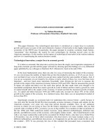
Fig. 3. Granger causality relationship flows.

another short-run bi-directional Granger causality, between energy
consumption and CO2 emissions. This implies that an increase in
energy consumption may increase carbon emissions and vice versa.
Energy consumption causes economic growth in the short-run in
Malaysia, Philippines and Thailand but the inverse is not true. The
results of granger causality movements are summarized in Fig. 3.

4. Conclusion
This study examines the cointegration and causal relationship
between economic growth, carbon dioxide (CO2) emissions and
energy consumption in five selected ASEAN countries namely
Indonesia, Malaysia, Philippines, Singapore and Thailand during
the period 1971e2008. The recently ARDL methodology proposed by Pesaran and Shin [39] and Pesaran et al. [40], and
Granger causality test based on VECM are employed. The study
established cointegration relationship between carbon emissions, energy consumption and economic growth in all the
countries with positive and statistically significant relationship
between carbon emissions and energy consumption in both short
and long-run.

Production of industrial output and evolution toward exportoriented technologies in ASEAN countries put more pressures on
the amount of energy consumed. About 90% of the ASEANs primary
commercial energy requirement is fulfilled by fossil fuels such as
coal, oil, and gas. This may lead to more emissions which in turn
will make the need for pollution control actions more urgent.
Furthermore following Narayan and Narayan [56] the long-run
elasticities of energy consumption variable with respect to carbon
emissions are higher than the short-run elasticities. This implies
that carbon emissions level is found to increase in respect to energy
consumption over time in the selected ASEAN countries.
Under the long-run analysis, there is a positive long-run elasticity
estimate of carbon emissions with respect to real GDP per capita and
a negative long-run elasticity estimate of carbon emissions with
respect to the square of per capita real GDP at 1% significance level in
Singapore, 10% significance level in the case of Thailand and statistically insignificance in the case of Malaysia. The long-run results
indicate that there is a negative long-run elasticity estimate of carbon emissions with respect to real GDP per capita and a positive
long-run elasticity estimate of carbon emissions with respect to the
square of per capita real GDP at 10% significance level in the cases of

Indonesia and Philippine. The finding implies that over time income


822

B. Saboori, J. Sulaiman / Energy 55 (2013) 813e822

contributes to less carbon dioxide emissions only in cases of
Singapore and Thailand. Furthermore Indonesia and Philippines are
still in the increasing part of the carbon Kuznets curve. This mixed
finding is expected, given the fact that these five selected ASEAN
countries are not at the same level of economic development and
economic development is not even throughout the region.
The results of short-run confirms the existence of EKC only in the
case of Thailand as the related coefficients to LY and (LY)2 are positive and significant at 1% and negative and significant at 5% significance level respectively. The underlying models also passed the
diagnostic tests for normality and functional form. Stability of the
short-run as well as long-run coefficients by applying the CUSUM
and CUSUMSQ tests proposed by Brown et al. [48] were also tested.
The stability of the variables in the estimated models suggests that
all the estimated models are stable over the study period.
The granger causality results suggest three long-run bi-directional Granger causality relationships between the variables. The
first one is a bi-directional Granger causality between energy consumption and CO2 emissions in all five ASEAN countries under
study. This suggests that carbon emissions and energy consumption
are highly interrelated to each other. The second and third bidirectional Granger causality relationships are between economic
growth and CO2 emissions and economic growth and energy consumption in Indonesia, Malaysia and Philippine. Furthermore, there
exists evidence of short-run bi-directional Granger causality between economic growth and CO2 emissions in Indonesia, Singapore
and Thailand. In the cases of Malaysia and Singapore there exists
another short-run bi-directional Granger causality, between energy
consumption and CO2 emissions. This implies that an increase in
energy consumption gives rise to more carbon emissions and vice

versa. Energy consumption causes economic growth in the shortrun in Malaysia, Philippines and Thailand but the inverse is not true.
References
[1] Shafik N, Bandyopadhyay S. Economic growth and environmental quality:
time series and cross-country evidence. World Bank working paper no. 904
1992. Washington, DC.
[2] Seldon T, Song D. Environmental quality and development: is there a Kuznets
curve for air pollution emissions. J Environ Econ Manage 1994;27:147e62.
[3] Unruh GC, Moomaw WR. An alternative analysis of apparent EKC-type transitions. Ecol Econ 1998;25:221e9.
[4] Galeotti M, Lanza A. Richer and cleaner? A study on carbon dioxide emissions
in developing countries. Energy Policy 1999;27:565e73.
[5] Dinda S, Coondoo D. Income and emission: a panel-data based cointegration
analysis. Ecol Econ 2006;57:167e81.
[6] Managi S, Jena PR. Environmental productivity and Kuznets curve in India.
Ecol Econ 2008;65:432e40.
[7] Shafik N. Economic development and environmental quality: and econometric
analysis. Oxf Econ Pap 1994;46:757e73.
[8] Cole MA, Rayner AJ, Bates JM. The environmental Kuznets curve: an empirical
analysis. Environ Dev Econ 1997;2(4):401e16.
[9] de Bruyn SM, van den Bergh JCJM, Opschoor JB. Economic growth and emissions: reconsidering the empirical basis of environmental Kuznets curves. Ecol
Econ 1998;25:161e75.
[10] Roca J, Padilla E, Farre M, Galletto V. Economic growth and atmospheric
pollution in Spain: discussing the environmental Kuznets curve hypothesis.
Ecol Econ 2001;39:85e99.
[11] Coondoo D, Dinda S. The carbon dioxide emission and income: a temporal
analysis of cross-country distributional patterns. Ecol Econ 2008;65:375e85.
[12] Akbostanci E, Turut-Asik S, Tunc GI. The relationship between income and
environment in Turkey: is there an environmental Kuznets curve? Energy
Policy 2009;37:861e7.
[13] Stern D. The rise and fall of the environmental Kuznets curve. World Dev
2004;32:1419e39.

[14] Dinda S. Environmental Kuznets curve hypothesis: a survey. Ecol Econ
2004;49:431e55.
[15] Kijima M, Nishide K, Ohyama A. Economic models for the EKC: a survey. J Econ
Dyn Control 2010;34:1187e201.
[16] Kraft J, Kraft A. On the relationship between energy and GNP. J Energy Dev
1978;3:401e3.
[17] Ozturk I. A literature survey on energyegrowth nexus. Energy Policy 2010;38:
340e9.

View publication stats

[18] Payne JE. Survey of the international evidence on the causal relationship
between energy consumption and growth. J Econ Stud 2010;37:53e95.
[19] Al-mulali U. Oil consumption, CO2 emission and economic growth in MENA
countries. Energy 2011;36:6165e71.
[20] Fallahi F. Causal relationship between energy consumption (EC) and GDP: a
Markov-switching (MS) causality. Energy 2011;36:4165e70.
[21] Ang JB. CO2 emissions, energy consumption, and output in France. Energy
Policy 2007;35:4772e8.
[22] Soytas U, Sari R, Ewing BT. Energy consumption, income, and carbon emissions in the United States. Ecol Econ 2007;62:482e9.
[23] Acaravci A, Ozturk I. On the relationship between energy consumption, CO2
emissions and economic growth in Europe. Energy 2010;35:5412e20.
[24] Ang JB. Economic development, pollutant emissions and energy consumption
in Malaysia. J Pol Model 2008;30:271e8.
[25] Zhang XP, Cheng XM. Energy consumption, carbon emissions, and economic
growth in China. Ecol Econ 2009;68:2706e12.
[26] Ghosh S. Examining carbon emissions economic growth nexus for India: a
multivariate cointegration approach. Energy Policy 2010;38:3008e14.
[27] Lotfalipour M, Falahi M, Ashena M. Economic growth, CO2 emissions, and
fossil fuels consumption in Iran. Energy 2010;35:5115e20.

[28] Menyah K, Rufael Y. Energy consumption, pollutant emissions and economic
growth in South Africa. Energy Econ 2010;32:1374e82.
[29] Ozturk I, Acaravci A. CO2 emissions, energy consumption and economic
growth in Turkey. Renew Sustain Energy Rev 2010;14:3220e5.
[30] Apergis N, Payne J. CO2 emissions, energy usage and output in Central
America. Energy Policy 2009;37:3282e6.
[31] Apergis N, Payne JE. The emissions, energy consumption, and growth nexus:
evidence from the common wealth of independent states. Energy Policy
2010;38:650e5.
[32] Lean H, Smyth R. CO2 emissions, electricity consumption and output in
ASEAN. Appl Energy 2010;87:1858e64.
[33] Pao H, Tsai C. CO2 emissions, energy consumption and economic growth in
BRIC countries. Energy Policy 2010;38:850e60.
[34] Al-mulali U, Binti Che Sab CH. The impact of energy consumption and CO2
emission on the economic growth and financial development of in the Sub
Saharan African countries. Energy 2012;39:180e6.
[35] Bashiri Behmiri N, Pires Manso JR. Crude oil conservation policy hypothesis in
OECD (organisation for economic cooperation and development) countries: a
multivariate panel Granger causality test. Energy 2012;43:253e60.
[36] Luzzati T, Orsini M. Investigating the energy-environmental Kuznets curve.
Energy 2009;34:291e300.
[37] Third ASEAN energy outlook. Japan: The Energy Data and Modelling
Center, The Institute of Energy Economics. />filemanager/2012/06/14/t/3/t3aeo-complete-outlook.pdf; 2010.
[38] Tanaka N. World energy outlook. International Energy Agency. http://www.
iea.org/speech/2010/Tanaka/weo_2010_beijing.pdf; 2010.
[39] Pesaran MH, Shin Y. An autoregressive distributed lag modeling approach to
cointegration analysis. In: Strom S, editor. Econometrics and economic theory
in 20th century: the Ragnar Frisch Centennial symposium. Cambridge:
Cambridge University Press; 1999 [chapter 11].
[40] Pesaran MH, Shin Y, Smith RJ. Bounds testing approaches to the analysis of

level relationships. J Appl Econ 2001;16:289e326.
[41] Halicioglu F. An econometric study of CO2 emissions, energy consumption,
income and foreign trade in Turkey. Energy Policy 2009;37:1156e64.
[42] Sari R, Soytas U. Are global warming and economic growth combatable? Evidence from five OPEC countries. Appl Energy 2009;86:1887e93.
[43] Engle RF, Granger CWJ. Co-integration and error correction: representation,
estimation, and testing. Econometrica 1987;55:251e76.
[44] Johansen S, Juselius K. Maximum likelihood estimation and inferences on
cointegration with approach. Oxford Bull Econom Stat 1990;52:169e209.
[45] Pesaran MH, Pesaran B. Working with Microfit 4.0: interactive econometric
analysis. Oxford: Oxford University Press; 1997.
[46] Narayan PK. The saving and investment nexus for China: evidence from
cointegration tests. Appl Econ 2005;37:1979e90.
[47] Bahmani-Oskooee M, Goswami GG. Exchange rate sensitivity of Japan’s
bilateral trade flows. Japan World Econ 2004;16:1e15.
[48] Brown R, Durbin J, Evans J. Techniques for testing the constancy of regression
relationships over time. J Roy Stat Soc B 1975;37:149e72.
[49] Dickey DA, Fuller WA. Likelihood ratio statistics for autoregressive time series
with a unit root. Econometrica 1981;49:1057e72.
[50] Philips P, Perron P. Testing for a unit root in time series regression. Biometrika
1988;75:335e46.
[51] Ouattara B. Aid, debt and fiscal policies in Senegal. J Int Dev 2006;18:1105e22.
[52] Kremers JJ, Ericson NR, Dolado JJ. The power of cointegration tests. Oxf Bull
Econ Stat 1992;54:325e47.
[53] Poa H, Yu H, Yang Y. Modeling the CO2 emissions, energy use, and economic
growth in Russia. Energy 2011:1e7.
[54] Chang C. A multivariate causality test of carbon dioxide emissions, energy
consumption and economic growth in China. Appl Energy 2010;87:3533e7.
[55] Pao H, Tsai C. Modeling and forecasting the CO2 emissions, energy consumption,
and economic growth in Brazil. Energy 2011;36:2450e8.
[56] Narayan PK, Narayan S. Carbon dioxide and economic growth:

panel data evidence from developing countries. Energy Policy 2010;38:661e6.