Theory of Partial Differential Equations

Theory of
Partial Differential Equations


This is Volume 93 in
MATHEMATICS IN SCIENCE AND ENGINEERING
A series of monographs and textbooks
Edited by RICHARD BELLMAN, University of Southern California
The complete listing of books in this series is available from the Publisher
upon request.


Theory of
Partial Differential Equations
H. M E L V I N LIEBERSTEIN
Department of Mathematics
University of Newcastle
Newcastle, New South Wales
Australia

@

ACADEMIC PRESS

New Yorkand London

1972


COPYRIGHT

0 1972, BY ACADEMIC
PRESS,INC.

ALL RIGHTS RESERVED
NO PART OF THIS BOOK MAY BE REPRODUCED IN ANY FORM,
BY PHOTOSTAT, MICROFILM, RETRIEVAL SYSTEM, OR ANY
OTHER MEANS. WITHOUT WRITTEN PERMISSION FROM
THE PUBLISHERS.

ACADEMIC PRESS, INC.
111 Fifth Avenue, N e w

York, N e w York 10003

United Kingdom Edition published by
ACADEMIC PRESS, INC. (LONDON) LTD.
24/28 Oval Road. London NWI

LIBRARY
OF CONGRESS
CATALOG
CARDNUMBER: 72-84278
AMS (MOS) 1970 Subject Classifications: 35-01, 35-02,
32A05, 65-01,95-02
PRINTED IN THE UNITED STATES OF AMERICA


Contents

xi

PREFACE

PART I . AN OUTLINE

Chapter I

The Theory of Characteristics, Classification, and
the Wave Equation in E 2
1.

2.
3.
4.
5.

6.

7.
Chapter 2

D’Alembert Solution of the Cauchy Problem for the
Homogeneous Wave Equation in E Z
Nomenclature
Theory of Characteristics and Type Classification
for Equations in E Z
Considerations Special to Nonlinear Cases
Compatibility Relations and the Finite-Difference
Method of Characteristics
Systems Larger Than Two by Two

Flow and Transmission Line Equations

3
8
12
17

18
21
22

Various Boundary-Value Problems for the
Homogeneous Wave Equation in E 2
1.
2.
3.
4.

The Cauchy or Initial-Value Problem
The Characteristic Boundary-Value Problem
The Mixed Boundary-Value Problem
The Goursat Problem

29
29
32
33
V

CONTENTS

5. The Vibrating String Problem
6. Uniqueness of the Vibrating String Problem
7. The Dirichlet Problem for the Wave Equation?
Chapter 3

Various Boundary-Value Problems for the Laplace
Equation in E 2
1. The Dirichlet Problem
2. Relation to Analytic Functions of a Complex Variable
3. Solution of the Dirichlet Problem on a Circle
4. Uniqueness for Regular Solutions of the Dirichlet
and Neuniann Problem on a Rectangle
5. Approximation Methods for the Dirichlet Problem
in E 2
6. The Cauchy Problem for the Laplace Equation

Chapter 4

The Slab Problem
An Alternative Proof of Uniqueness
Solution by Separation of Variables
Instability for Negative Times
Cauchy Problem on the Infinite Line
Unique Continuation
Poiseuille Flow
Mean-Square Asymptotic Uniqueness
Solution of a Dirichlet Problem for an Equation of
Parabolic Type

51

53
56

59
61
62
62
63
65
66
69
71

Expectations for Well-Posed Problems
1. Sense of Hadamard
2. Expectations
3. Boundary-Value Problems for Equations of EllipticParabolic Type
4. Existence as the Limit of Regular Solutions
5. The Impulse Problem as a Prototype of a Solution
in Terms of Distributions
6. The Green Identities
7. The Generalized Green Identity
8. .P-Weak Solutions
9. Prospectus
10. The Tricomi Problem

vi

45
47
50

Various Boundary-Value Problems for Simple
Equations of Parabolic Type
1.
2.
3.
4.
5.
6.
7.
8.
9.

Chapter 5

36
40
42

73
75
82
84
85
87
89

91
93
94


CONTENTS
PART 11. SOME CLASSICAL RESULTS FOR NONLINEAR
EQUATIONS IN TWO INDEPENDENT VARIABLES

Chapter 6

Existence and Uniqueness Considerations for the
Nonhomogeneous Wave Equation in E Z
Notation
Existence for the Characteristic Problem
Comments on Continuous Dependence and Error Bounds
An Example Where the Theorem as Stated Does Not
Apply
5. A Theoremusing the Lipschitz Condition on a Bounded
Region in E 5
6. Existence Theorem for the Cauchy Problem of the
Nonhomogeneous (Nonlinear) Wave Equation in E 2

1.
2.
3.
4.

Chapter 7

Characteristic Boundary-Value Problem
Determination of the Riemann Function for a Class
of Self-Adjoint Cases
5. An Integral Representation of the Solution of the
Cauchy Problem

4.

112
114

118
120
124
126
128

Classical Transmission Line Theory
The Transmission Line Equations
The Kelvin r-c Line
Pure I-c Line
Heaviside’s r-c-l-g Distortion-Free Balanced Line
Contribution of Du Boise-Reymond and Picard to
the Heaviside Position
6. Realization
7. Neurons

1.
2.
3.

4.
5.

Chapter 9

110

The Riemann Method
1. Three Forms of the Generalized Green Identity
2. Riemann’s Function
3. An Integral Representation of the Solution of the

Chapter 8

101
102
110

131
133
136
137
139
140
141

The Cauchy-Kovalevski Theorem
1. Preliminaries; Multiple Series
2. Theorem Statement and Comments
3. Simplification and Restatement

4. Uniqueness
5. The first Majorant Problem

142
145
148
149
150

vii


CONTENTS
6.
7.

An Ordinary Differential Equation Problem

Remarks and Interpretations

151
153

PART 111. SOME CLASSICAL RESULTS FOR THE LAPLACE AND
WAVE EQUATIONS IN HIGHER-DIMENSIONAL SPACE

Chapter 10 A Sketch of Potential Theory
1.
2.
3.

4.
5.
6.
7.
8.
9.
10.
11.

Chapter 1 1

Uniqueness of the Dirichlet Problemusing the
Divergence Theorem
The Third Green Identity in E 3
Uses of the Third Identity and Its Derivation for
En,n#3
The Green Function
Representation Theorems Using the Green Function
Variational Methods
Description of Torsional Rigidity
Description of Electrostatic Capacitance, Polarization,
and Virtual Mass
The Dirichlet Integral as a Quadratic Functional
Dirichlet and Thompson Principles for Some Physical
Entities
Eigenvalues as Quadratic Functionals

159
160

165
166
167
169
170
171
172
174
175

Solution of the Cauchy Problem for the Wave
Equation in Terms of Retarded Potentials
1. Introduction
2. Kirchhoff's Formula
3. Solution of the Cauchy Problem
4. The Solution in Mean-Value Form
5. Verification of the Solution of the Homogeneous Wave

Equation
Verification of the Solution to the Homogeneous
Boundary-Value Problem
7. The Hadamard Method of Descent
8. The Huyghens Principle

6.

177
178
183
185

186
187
189
193

PART IV. BOUNDARY-VALUE PROBLEMS FOR EQUATIONS OF
ELLIPTIC-PARABOLIC TYPE

Chapter 12 A Priori Inequalities
1. Some Preliminaries
2. A Property of Semidefinite Quadratic Forms

...

Vlll

20 1
203


CONTENTS

3. The Generalized Green Identity Using u
4. A First Maximum Principle
5. A Second Maximum Principle
Chapter 13

= (u2 +

C ~ ) P / ~

204
207
210

Uniqueness of Regular Solutions and Error Bounds
in Numerical Approximation
1.
2.
3.
4.
5.

A Combined Maximum Principle
Uniqueness of Regular Solutions
Error Bounds in Maximum Norm
Error Bounds in Lp-Norm
Computable Bounds for the LZ-Normof an Error
Function

215
216
216
218
219

Chapter 14 Some Functional Analysis

1.
2.

3.
4.
5.
6.
7.
Chapter 15

General Preliminaries
The Hahn-Banach Theorem, Sublinear Case
Normed Spaces and Continuous Linear Operators
Banach Spaces
The Hahn-Banach Theorem for Normed Spaces
Factor Spaces
Statement (Only) of the Closed Graph Theorem

22 I
225
230
233
235
238
239

Existence of z p - W e a k Solutions
A First Form of the Abstract Existence Principle
I ) ; Riesz Representation
Function Spaces gPand 2’p‘(pA Reformulation of the Abstract Existence Principle
Application of the Reformulated Principle to =.Yp-Weak
Existence
5. Uniqueness of 2”’-Weak Solutions

6. Prospectus

1.
2.
3.
4.

240
244
245
246
248
249

NOTES

253

REFERENCES

264

INDEX

267

ix


This page intentionally left blank

Preface

This book is written in four modular parts intended as easy steps for the student.
The intention here is to lead him from an elementary level to a level of modern
analysis research. Thus the first pages of Part I are an explanation of the regular
(classical) solutions of the second-order wave equation in two-space-time, while
the latter pages of Part IV encompass a more or less complete analysis of the existence of dLPP-weak solutions for boundary-value problems for equations of ellipticparabolic type expounded according to G. Fichera of the University of Rome. In
the developing process, an effort is made to ensure that the student samples the
extensive variety of mathematically conceivable boundary-value problems, even if
their properties are not entirely satisfying once analyzed, and that he learns how to
use these tools to elucidate phenomena of nature and technology.
The field is to some extent characterized by the fact that one rarely “solves”
boundary-value problems in any acceptable sense of the word. Since computing
plays an altogether inseparable role in approximating solutions to boundary-value
problems, we present wherever possible a skeleton of the basic theoretical framework
for the numerical analysis of several problems along with that of the theory of
existence, uniqueness, and integral representations. Where numerical techniques
are thought to be suggestive, we present them before presenting existence-uniqueness
theories; sometimes when useful and not grossly misleading, we may even present
them in lieu of existence-uniqueness theories. Also, we occasionally interrupt other
presentations to give some theoretical background of basic computational procedures. However, any serious presentation of the theory of computation procedures
is beyond the scope of this book. Nevertheless, we still have tried to present a text
in which there is a natural integration of the topics of existence, uniqueness, approximation, and some analysis of computation procedures with applications.

xi


PREFACE

Actually, our purpose has been to write a readable and teachable general text of
modern mathematical science-ne
without substantial pretext to technical originality and yet one that is exciting and thorough enough to provide a basic background.
The advantage of the modular approach is that a student may start where he finds
his level, stop where his interests stop, and continue at his own rate, even piecemeal
if he is so inclined. Courses can easily be organized from the text in the same manner.
An instructor will find that he can easily addend or delete material without destroying the continuity of presentation. We believe, in fact, that most instructors want a
text that will help them to organize their own course rather one that demands a
specific approach. From our experience, we can recommend the following organizations of courses from this text, but we hope other instructors will find their own
useful combinations of material and perhaps insert their own favorite topics:
Mode 1: Part I, only-a one-quarter course for students of engineering and
physics,
Mode 2: Parts I and 11-a one-semester, first-year graduate or senior-level
course for students of mathematics, engineering, and physics,
Mode 3 : Parts I-111-a
two-quarter, first-year graduate or senior-level course
for students of mathematics, engineering, and physics,
Mode 4: Parts I-IV-a
two-semester, or three-quarter, first-year graduate or
senior-level course for students of mathematics, engineering, and
physics,
Mode 5 : Parts I-IV-a two-quarter (only) course at the third-year graduate level
in mathematics (at this level, portions that review functional analysis,
for example, can be skipped).
We have found it more pretentious than useful to present here a rCsume of
Lebesgue integration theory, but have, nevertheless, included a treatment of functional analysis that is fairly complete up to the point where it is required for our
presentations. We believe the treatment is as brief and readable as one can find
useful in the field. Except for our failure to present Lebesgue integration theory,
which is really needed only in the last chapter (and even that can be bravely faced

without it), we have kept our prerequisites down to just some introductory analysis
beyond the level of the usual elementary calculus course and some elementary
linear algebra. However, the instructor operating in Mode 1 may choose to dispense
with even this requirement. I have taught these materials in Modes 1, 2, and 4.
Professor Charles Bryan of the University of Montana, who as a doctoral student
under my direction helped to write Chapter 15, has successfully used the materials
from this text in Mode 5 (during 1969-1970). His assistance with the writing of this
book has been most valuable, and Mode 5 is his idea. We must also acknowledge
the influence of Professor Bernard Marcus of San Diego State College in the functional analysis chapter and Professor Robert Stevens of Montana University for a
certain example we have used in Chapter 6 ; at the time when their contributions
were made, both were engaged in doctoral studies under my direction.

xii


PREFACE

The Mode 3 presentation does not involve Lebesgue integration beyond the level
of some comments, mostly restricted to notes collected at the end of the text.
We have conceived Part I to be our “outline.” Here we encourage the student to
seek an understanding of the entire field of boundary-value problems by way of a
more or less exhaustive study of the simplest linear homogeneous equations of the
second order in two independent variables. This material must be completely understood before passing on to the study of the intensively analytic theorems of extensive
generality that we find characterizes mature knowledge in this field. Our “outline”
material is intended to provide breadth, not depth which, from our point of view,
can only come in stages. Simply, successive parts of the book are designed to help in
achieving successive levels.
Part I1 treats of existence and uniqueness by way of Picard iteration of the charteristic and Cauchy (initial value) problems for the wave equation in E Z with its
nonhomogeneous part depending, in a possibly nonlinear way, on the solution and
its first partial derivatives. The Riemann method is developed, giving nonsingular

integral representations for the linear case. This would seem to represent one of the
admirable direct achievements of classical analysis, apparently motivated by
Riemann’s desire to understand flows of materials under large impact loadings and
almost immediately applied by others to achieve an understanding of balanced
transmission lines, foreshadowing the advent of clear long distance voice telephony.
Transmission lines are studied in a separate chapter in Part 11. Part I1 also treats
the Cauchy-Kovalevsky theorem, which concerns analytic solutions of analytic
equations corresponding to analytic data on a segment of an analytic initial value
curve. The setting of Part I 1 is thoroughly classical in conception throughout. It
is quite important and unavoidably difficult in spots, even though it involves no
advanced prerequisites.
In Part I l l we first sketch classical potential theory,* including the usual integral
representations for the solution of the Dirichlet problem in terms of the Green
function in n dimensions and a somewhat modern approach to variational principles
for estimating quadratic functionals. The latter includes studies of such diverse
topics as torsional rigidity and bounds for eigenvalues associated with some of the
important boundary-value problems. It is then possible to move with ease to a study
of the wave equation in higher dimensions, where the intriguing beauty of the
Huyghens principle is emphasized and its inner workings exposed by using the
Hadamard method of descent. Classical analysis eventually became heavily burdened
with clever but extensive and delicate manipulations-presumably this overburden
on analysis caused functional analysis to be conceived-and the latter portions of
Part 111 unavoidably reflect this heavy manipulative style, but again it involves no
advanced prerequisites.
Part 1V presents a resume of functional analysis, develops several a priori estimates
for equations of elliptic-parabolic type (second order, n dimensions) from the
*This topic was once a semester or even year graduate course in mathematics.

...

XI11


PREFACE

divergence theorem, uses these to prove uniqueness of certain boundary-value problems, generates bounds therefrom for errors of approximation, and finally develops
an Abstract Existence Principle, which is used to prove the existence of YPP-weak
solutions. This last assumes, but does not require, a rudimentary knowledge of
Lebesgue integration theory. Part I V is intended to provide in very specific terms a
picture of the general techniques now being used in niodern studies of partial differential
equations. At the end of Part IV, a discourse is undertaken concerning various modern
senses of existence. Their physical relevance is reviewed, perhaps too briefly, but to
the best of our ability. This is found to suggest apossibility that it isperhaps primarily
the sense of uniqueness that we should think now to weaken-perhaps we should
weaken it to time-asymptotic uniqueness with a quickly acquired (unique) steady
state-retaining our classical (regular) sense of existence and at the same time insisting that all applied problems be treated as time dependent and not as stationary. If
there is any technical, as opposed to expository, originality to be claimed for this
text, it is the development of this thesis. We have tried, however, not to impose a
private view onto a public body, simply asking that an awareness of such issues and
an open mind concerning them be maintained. These, after all, are the issues raised
in the last 20 years of progress in partial differential equations, and the effect of
these 20 years has been so profound that the thinking in the field will never be the
same again.
Perhaps the field of partial differential equations has suffered from too intense
specialization among its adherents in the last several generations, but the danger now
is too much generality taken on too fast by students without sufficient grounding in
“real problems.” We have tried here to introduce increased generality at a modest
rate of increasing abstraction in stages that would seem to develop its justification in
terms of problems that appear to be “real” at each stage.
Notes of general scientific and historical interest are collected at the end of the

book (keyed to sections of various chapters) in order not to interrupt the flow of
mathematical developments.

xi v


P A R T

I

An Outline


This page intentionally left blank


C H A P T E R

1

The Theory of Characteristics,
Classification, and the Wave Equation in EL

1 D'ALEMBERT SOLUTION OF THE CAUCHY PROBLEM FOR THE
HOMOGENEOUS WAVE EQUATION IN EZ

Let us consider under what conditions it is possible to determine a unique
solution of the equation
u,,

- uyy= 0

(1.1.1)

and

(1.1.2)

satisfying the conditions
u(x,O) = f(x)

uy(x,O) = g(x)

where f: ( a , b ) + R ' and g: (a,b)+ R'. We understand that as part of this
task we are to decide precisely what we wish to mean by saying a function u
is a solution of (l.l.l), (1.1.2) and what properties given functions f and g
must have so that such a solution exists and is unique. Toward this end we
rewrite Eq. ( I .l.1) in coordinates rotated through 4 5 O ,

5

=t(x

+Y ) ,

rl = t ( x - Y ) ,

( 1.1.3)

by the use of the chain rule on the function u. Let us remark here once and for

all that there are really two functions involved, one a function of x and y,
another a function of 5 and formed as a composite of the first with (1.1.3),
) (5, q )
both of which have the same functional values at those points ( x , ~and

3


I . T H E T H E O R Y OF C H A R A C T E R I S T I C S

which are identified by (1.1.3). Because of this sameness of functional values
arising by the formation of composite functions, we will use the same symbol
u for both functions. Thus we may write u ( . ~ , yor
) u ( 4 , q ) for functional
values if the distinction of which function is used is not otherwise clear by
the context, but the one symbol u will be used for both functions. Far from
leading to confusion, as long as we agree to what is being done, this will help
keep our bookkeeping straight as to which functional values are to be
identified. This will be especially useful if we encounter long strings of changes
of variables as one very often does in extensive application areas. As far as
we know, all textbooks in partial differential equations are written using this
convention, but in these times when the distinction between functions and
their functional values is being greatly emphasized even in elementary training
it would seem to need statement. In any case, it will be used throughout this
text and not mentioned again unless clarification seems specifically demanded
by the nature of the arguments presented.
From the chain rule we have

=

t@<<
+ u,lq)- 3u<,

so that (1. I . 1) becomes
U<,( =

0.

(1.1.4)

~ u , are
~ ~continuous and are therefore
Here it has been assumed that u < ,and
equal; i.e., we are now restricted to seek a solution with this property.
We now seek the class of all solutions of (1.1.4). Equation (1.1.4) implies
that uy is a function of 4 alone. If this function is integrable, then we may
write
(1.1.5)

where G is an arbitrary function of I ] introduced by this last “integration”
and F, being the primitive of ut (a function of 4 alone), is also arbitrary.
We have thus shown that all solutions of (1.1.4) such that uE,is integrable
are of the form (1.1.5). Now we must ask if all forms (1.1.5) are solutions of
4


1. D’ALEMBERT SOLUTION OF THE CAUCHY PROBLEM

(1.1.4). The question resolves to, what do we mean by a solution? Here we
simply ask that all terms specifying quantities in (1.1.4) exist in some region R

where this question is to be resolved and that (1.1.4) be satisfied in that region.
But since we ask for an equality to be satisfied, we will also ask that all terms
in the equation be continuous-here that uy, be continuous in the region of
consideration. It is evident that the function u as given in (1.1.5) is a solution
in this very concrete sense if F, G E C’ on sufficiently large open intervals
of 5 and y ~ .
Reverting back to the original coordinates, we have from (1.1.5)
U(X,Y) =

F(x+y)

+ G(x-y),

( 1.1.6)

where the definitions of F and G have been altered to absorb the factor 4 in
the arguments. Here u is a solution of (1.1.1) in the sense that all terms exist
and are continuous in a region of consideration if F, G E C2, and, moreover,
if F, G E C2(a,b), then one can see that u E C z ( T ) where T is an isosceles
triangle built on the base (a, 6). Clarification of the latter will be undertaken
in a moment; for now, we should note that the properties required of F and G
in order that u in (1.1.5) be a solution in ( < , q ) coordinates are somewhat
weaker than the properties required of them in order that (1.1.6) be a solution
in (x,y) coordinates. This is a peculiar property of solutions of partial differential equations when considered in this very direct concrete sense, and it is
one of the reasons (not the most cogent, however) why many modern workers
prefer a more abstract sense of the existence of solutions. Such workers will
be seen to lose much, however, in the way of useful physical interpretations
of their results when they weaken the sense of existence. A balanced consideration of whether one should use the concrete sense (regular solutions, as
we call them) or an abstract sense (e.g., YP-weak solutions) of the existence of
solutions is a theme that will be threaded through this text but it has little

relevance yet, and at first we are compelled to consider only the concrete sense
of solutions. To some extent, where possible, it will be found that we prefer
to weaken the sense of uniqueness rather than existence. Again that is far
ahead of the story.
To find F a n d G in (1.1.6) so that (1.1.2) is satisfied we put

f(x) = F(x) + G(x)

(1.1.7)

and
g(X)

=

F’(x) - G’(x)

(1.1.8)

where F ( x + y ) and G ( x - y ) have been differentiated as composite functions of
x and y and then y has been put equal to zero. Letting c be any real number,
5


1 . T H E THEORY OF CHARACTERISTICS

and assuming g is integrable, ( I . 1.8) can be written

/‘b@)ds

=

( 1 .1.9)

F ( x ) - G(x).

Then from (1.1.7) and (1.1.9),

( I . I . 10)
and

“ I* 3

G(x) = - f ( x ) -

2

g(s)ds

.

(1.1.11)

These are functions of one variable, but this one variable appears as functional
values of two different functions of two variables in ( I . 1.6), both as x + y and
x - y . With this in mind we see that (1.1.6) becomes
U(X?Y) =

+L-f(x+u)+f(x-r)I

+ + / x + y g ( s )ds

( 1.1.12)

x-Y

where it is also seen that the arbitrary reference value c no longer appears.
This, i.e. (1.1.12), is what we refer toas the D’Alembert solution. D’Alembert
is one of our classical fountainheads, so this solution is hardly recent. It
provides us with a starting or reference point from which to depart for an
understanding of many things. But is it a solution in our concrete sense,
and if so, in what region? One sees immediately that (1.1.2) is satisfied and
that (1.1.12) is of the form (1.1.6); a quick glance shows that u can be twice
continuously differentiated wherever f can be and where g can be once continuously differentiated.
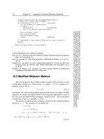
Y

-

x -y =const

6

FIG. 1 The solution is uniquely
determined in the triangle bounded by
y = 0, x--y= const, and x + y = const.


1 . D'ALEMBERT SOLUTION OF T H E C A U C H Y PROBLEM

Let us select a point (x,y) (see Fig. 1) and ask about the value of u at this

point. Draw a line through this point so that x + y is constant and another so
that x - y is constant, and note where these lines cross the x axis. There we
pick up the valuesf(x+y) andf(x-y) to use in (1.1.12). Also, the integral
term in (1.1.12) is just the integral of g between these points of intersection.
From Fig. 1 , then, with the comments in the paragraph above, it becomes
clear that D'Alembert solution (1.1.12) is indeed a solution in our concrete
(regular) sense in the 4.5' isosceles triangle T with base (a,b) i f f € CZ(a,b)
and g E C'(a, 6).
But is the D'Alembert solution a unique regular solution? Before undertaking this question let us record just what it is that we have now decided to
call a regular solution: Let T be an open 4.5' isosceles triangle with base
(a,6) on the x axis. If u : T + R' and
(i) u € C 2 ( T ) ;
(ii) u E C ( T u (a,6));
(iii) (1.1.1) is satisfied for every (x, y ) E T ; and
(iv) (1.1.2) is satisfied for every x E (a,6);
then u is said to be a regular solution of ( 1 . 1 . I), (1.1.2) in T . Condition (ii)
provides a connection between the specification of the data as required by
(iv) on y = 0 and the specification of the differential equation as required by
(iii) in the (open) region' T. Some such condition will always be needed in
the specification of a boundary-value problem as one can see, but it will
sometimes be weakened when the boundary-value problem is restated as an
integral equation, and we will often strengthen it to u E C' in order to use the
divergence theorem conveniently in this outline.
Uniqueness is handled here, as it will always be handled for linear (see the
next section) problems, by a simple contradiction argument. Suppose there
are two regular solutions u , and u2 o f ( l . l . l ) , (1.1.2).Then
u

=

241 - u 2

satisfies the homogeneous equation

u,, - uyy = 0

(1.1.13)

u(x,O) = u,(x,O) = 0.

(1.1.14)

and the homogeneous data

t We will always mean by a region an open, connected set.
7


1. THE THEORY OF CHARACTERISTICS

We must show that (1.1.13) and (1.1.14) together imply that u = 0 for every
( x , y ) E T so that u1 and uz are equal on T. The problem (l.l.l3), (l.l.l4),
or an appropriate adaptation of it, is always the uniqueness problem for
linear equations, and we will not always feel compelled to mention this oftrepeated argument when it is being repeatedly used.
Here for the uniqueness problem we have the opportunity, exceedingly rare
in partial differential equations, to use the form (1.1.6) giving all regular
solutions. Obviously, (1.1.13), (1.1.14) require that F = G = 0 in (1.1.6) and
uniqueness is established.
The triangle T is called the “region of determination” of the interval (a, 6).
The “domain of dependence” D of a point ( x , ~ )is the base of an isosceles

triangle on the x axis with ( x , y ) as its apex. The “region of influence” R of
the interval (a, b) is the infinite region shown in Fig. 2 between x - y = 6 and
x + y = a. From (1.1.12) and the arguments given above, the student will
readily agree that these entities are well named.
Y

FIG.2
2 NOMENCLATURE

The term “linear” was used in connection with our discussion of uniqueness
before its meaning was stated here. To avoid such occurrences, we now
interrupt our substantive presentation to display some of the basic nomenclature in the field.
Let f:R*-+ R‘ (or possibly f: C 8 + C ’ ) . Then a second-order partial
differential equation for a function u : RZ-+ R‘ (or possibly u : C2-+ C’) is
an equation
(1.2.1)
f(x, Y , u, ux, uxx, uxy,uyy)= 0.
uy9

A definition for a higher-order (referring to the highest number of derivatives
of u appearing) equation and one involving more independent variables,
u : R” -+ R‘ for n > 2, can easily be rendered by the student. Invariably some
8


2. NOMENCLATURE

conditions onfwill be included in the statement of any particular problem or
theorem; it may be required that it be possible to solve (1.2.1) for uyyor that
f b e linear in uxx,uxy,uyyor even thatfbe linear in all but the first two entries,

x and y .
If .f is linear in the highest-order derivatives appearing, then the equation
(1.2.1) is described as “quasi linear.” In this case ( I .2. I ) can be written
a(x,y, u, u,, uy)u,,
=

4 x 9

Y , u,

+ 2&,

Y , u, uxr uy)uxy+ C ( . Y , Y , u,u,, uy)uyy

( I .2.2)

uy),

where a, b, c, d : R s -+ R ’ . The left member, the sum of highest-order terms
appearing, is called the principle part. This part will be found to play an
important role, telling us what curves are characteristic, as introduced in the
next section, and, therefore, what kinds of boundary-value problems are
proper and in what regions solutions are uniquely determined.
lffis linear in u and all its derivatives, then the differential equation is said
to be linear. In this case (1.2.1) can be written
a (x, Y ) uxx

+ 26 (x, Y ) u,y + c (-r,Y )u y y

= cc(&Y)

+ B(x,v)u + Y (.Y,Y) u, + 6 ( X . Y ) u y

( I .2.3)

where a, 6 , c, cc,fi, y , 6 : R 2+ R‘. If a, b, c,P, y , 6 E R‘ (i.e., w I , w,, w,, w4, w5, w6
R‘ and a : R‘ -+ { w , } , 6: R’ { w 2 } , c : R‘ + {w,}, B : R’ + {w,}, y : R‘ +
{w5}, 6: R‘ -+ {w,}), then (1.2.3) is said to be “of constant coefficients.” If
cc(x,y)=O for every (x,y) (in some region R of our consideration) then
(1.2.3) is said to be homogeneous; here u = 0 is a solution. The wave equation
( I . I. 1) is linear, homogeneous, and of constant coefficients. Its principle part
is called “the wave operator” and constitutes all nonzero terms of the equation.
We will find in Section 3 that the equation is “of hyperbolic type” and the
two families of “characteristics” are given by x + y = constant, the curves that
were found to bound the region of determination in Section 1. Moreover, we
will find that this was no accident but is to be expected as a general property
of hyperbolic type, and this serves to distinguish hyperbolic type. Of course,
in general, equations of constant coefficients are by far the easiest to understand, and in large measure our considerations of boundary-value problems
in this outline will be for equations of constant coefficients, mostly homogeneous ones. The linear case is much the easier to work with in theoretical
questions because the principle of superposition applies for the homogeneous
linear case: We leave it to the student to show that if u I and u2 are solutions
of the homogeneous equation (1.2.3) [i.e., with cc(x,y) = 0 for every ( x , y ) in
the region of consideration], then for m , n E R ’ , mul +nu, is a solution of
E

9


1 . THE THEORY OF CHARACTERISTICS

the same equation. This is the all-important principle of superposition ;
really it, rather than that f is linear, should be thought of as characterizing
linear equations.
Let Fi: R3”+’ -+R ’ , i = 1, ..., n. Then the n x n system of partial differential
equations
F1 (x,Y;u1, ..., un; u l , x , **., u n , x ; u1,y , Un,y) = 0
(1.2.4)
Fn(x,y; uI,...,un; u ~ , x , . . . , u n , x ; ul,y,*.*,un,y)= 0
is said to be a first-order system of partial differential equations in n realvalued functions u i : R2 + R’ of two real variables x , y . For purposes of
simplicity, we will often speak of the n = 2 case, though this will often have to
be followed by a discussion of complications arising in the general case.
When no such discussions follow, unless we are discussing a very specific
equation, the obvious generalizations apply and the n = 2 case is stated as a
prototype.
Following this approach, we now look at the quasi-linear case where, of
~ , q Y ,i = 1, ..., n ;
course, the functions Fi, i = 1 , ..., n, are linear in u ~ ,and
in the n = 2 case these equations are

a1 1 u,

+ a12 u y + b , 1 vx + 612 vy = h ,

a21 ux + a22 u y

+ 6 2 1 vx + 6 2 2 v y

(1.2.5)

= h2

where aij,b,,, hi: Rm+’+ R’. In the n x n case we can write
A U x + BUY= H

(1.2.6)

where A = ( a i j ( x , y ,ul,. .., u,,)) and B = ( b i j ( x , y ul,.
, .., un)) are n x n square
, u,,)) is a column
matrices of real-valued functions and H = ( h j ( x , y , u l ...,
matrix of real-valued functions. Of course, once again, if functions hj,
,j = 1, ..., n, are linear in u l , ..., u, and A and B are functions of (x,y) alone,
then (1.2.6) [or (1.2.5) with n = 21 is said to be linear; the functions F j ,
j = 1, ..., n, in (1.2.4) will be linear in functions u,, ujx,ujy,j = 1 , . .., n, and the
principle of superposition will apply for the homogeneous case. Of course,
“homogeneous” is now defined in an obvious way. If A and B are matrices
of constants and H i s a column matrix of functions
u(x,y)

+

rn
i= 1

Piui

where

pi E R ’ ,

then (1.2.6) is said to be “of constant coefficients.”
It will be important to notice in Section 3 and following that systems of
first-order equations are more general than one higher-order equation. This
10