Nghiên cứu giải pháp nâng cao khả năng chống nhiễu cho các bộ thu định vị GNSS tiên tiến robust signal processing techniques for modern GNSS receivers

INTRODUCTION
With the development of new navigation system (Galileo-European
system and BEIDOU-Chinese system), and the modernization of the
existing navigation system such as GPS and GLONASS, the positioning
performance of GNSS has been significantly improved. GNSS services
not only provide position but also provide high precise timescale for
synchronizing systems such as telecommunication and network.
Although they are widespread coverage of applications in many important
sectors, the signals and services of GNSS systems are highly sensitive to
malicious radio frequency interference (RFI) as well as jamming and
spoofing; meanwhile, the quality of such services is not guaranteed to the
conventional users. Technically, the GNSS signal is transmitted from
satellites away from Earth (about 20.000 km), so when it comes to
receivers, the signal power is smaller than the background noise about
1024 times (26dB) [1]. Therefore, any source of interference (jammer,
digital terrestrial communication systems, ionosphere scintillation) may
reduce the quality of the received signal, which in turn can disable the
operation of the receiver. In addition, because the GNSS systems are often
under the management of military based organizations [2] [3] [4], the
open services (e.g., GPS L1 C/A, Beidou B1, GLONASS L1OF) are
provided to users without any guarantee of the reliability.
Nowadays, ensuring reliable position and time information is essential in
many applications ranging from transport applications to emergency
applications. Hence, the modern receivers must be able to detect the
interference to determine the reliability of the position. In addition, the
position and time information must be available even where the GNSS
signal is not continuous.
A popular method for robust GNSS receiver performance is using
multiple physical antenna elements which is so-called as an antenna array.
This technique has been studied in the 1940’s with the widely using in the
radar and telecommunications applications [5] [6] [7] [8]. It is considered

as a promising method in GNSS receivers where spoofing, jamming and
interference are emerging threats. Although there are several studies in
using array-based processing for GNSS receivers [9] [10], there are
1


several existing issues involved to the implementation in a GNSS
receivers. Although using 2 bits in ADC is sufficient for GNSS receiver
[1], it makes the GNSS receivers less robust to the threats. Secondly, the
number of antenna elements is also limited due to the bandwidth of
interfaces. The existing antenna array frontend for GNSS receivers pack
all element samples into a single packet and send to digital processing
chains through a single interface.
A different method for robust GNSS receiver is the use of snapshot
positioning-based receiver (coarse-time positioning). It is considered as
an efficient method that can be applied to the area where the continuous
GNSS signal tracking is not guaranteed due to interference or jamming
[11] [12]. Recent studies have been improved its positioning performance
on the GPS L1 snapshot receiver [13] [14] [15] but the using multiconstellation and INS integration in snapshot receiver have not been
explored sufficiently in previous efforts.
Taking everything into account, the dissertation presents the robust signal
processing techniques for modern GNSS receivers. This thesis shows
how the synchronization issue in antenna array can be addressed to
expand the elements to unlimited number in theoretically. The technique
is also validated with both simulation and real data. Also, the dissertation
presents a complete solution from hardware to software of a multi-GNSS
snapshot receiver which can achieve a similar performance with a
traditional receiver while using few milliseconds of data. Also, through
the dissertation, all the simulations are conducted with the generated from
a software-based GNSS simulator. The design and implementation of this

simulator is introduced in this thesis.
This thesis results have been published 6 conferences and 5 journals as
listed in the attachment. The works have been carried on Hanoi University
of Science and Technology (Vietnam) and Politecnico di Torino (Italy)
Thesis outline
The thesis is organized in 4 chapters as follows:
Chapter 1 – Fundamental Background: In this chapter, the background
knowledge related to the stages of GNSS receiver architecture including:
acquisition, tracking and data demodulation, and position computation are
revised.
2


Chapter 2 - GNSS Signal Simulator Design and Implementation: In this
chapter, the design, implementation of a GNSS software-based simulator
are carefully considered. As one of the most important parameter related
to the speed of signal generation, the effect of sampling frequency is also
generalized theoretically in both simulator and receiver sides.
Chapter 3 – Antenna Array Signal Processing in GNSS Receivers: This
chapter focus on the solution enabling extending the number of elements
and the quantization bit. It is applied in a low-cost antenna array for
detecting the source of spoofing and interference
Chapter 4 – Snapshot Signal Processing in GNSS Receivers: This chapter
shows how the multi-constellation snapshot technique can be effectively
implemented. In addition, to improve positioning performance, the
snapshot GNSS/INS integration is proposed

3

1. FUNDAMENTAL
1.1. GNSS positioning principle
This section will explain the general principle of GNSS navigation.
Basically, GNSS positioning is based on trilateration techniques. In this
technique, the receiver firstly determines the distance from its position to
at least 3 known points. After that, the receiver’s position is determined
by the intersection of 3 sphere.
Let’s us denote 𝐮 = [𝑥𝑢 𝑦𝑢 𝑧𝑢 ] and 𝐱 𝑖 = [𝑥 𝑖 𝑦 𝑖 𝑧 𝑖 ] being the
position of the receiver and the satellite i. The geometry distance
from the receiver to satellite is defined as 𝑟 𝑖 = ||𝐮 − 𝐱 𝑖 ||. Clearly,
the vector 𝐮 can be determined if we know the satellite position 𝐱 and
the distance 𝑟
In GNSS receivers, the distance cannot be measured directly but it
uses the transmission time from satellite to receiver. Unfortunately,
the receiver clock is not synchronized with the atomic onboard of
GNSS satellites. As a result, we have one more unknown variable
𝛿𝑡𝑢 besides 3 unknown elements of 𝒖.
1.2. History and development of GNSS
1.3. GNSS Threats
1.4. GNSS Receiver Architecture
1.4.1.

Signal Conditioning and Sampling

The architecture of the signal conditioning and sampling is illustrated as
in the corresponding figure.
In this stage, the received signal is to condition to meet the requirement
of sampling process. For simplify, we consider the GPS L1 signal from a
satellite:
(1)

𝑠(𝑡) = √2𝑃𝑠 𝐶(𝑡 − 𝜏)𝐷(𝑡 − 𝜏)cos(2𝜋𝑓𝑠 𝑡 + 𝛷)
where 𝑃𝑠 is the received power of the GPS L1 signal. 𝐶(𝑡) and 𝐷(𝑡)
denotes the code and data of the consdired satellite.

4


After the mixer, the received signal is separated into I and Q
component. Without loss of generality, from now on, we will use the
complex signal to represent the signal on I and Q channel.
1.4.2.

Acquisition

The acquisition stage is aimed to roughly estimate the code phase and
Doppler shift of visible GNSS satellites. In fact, the stage performs
correlation with every Doppler frequency and code phase bin in the search
space. A satellite is considered as visible if there is the value of a cell in
the search space higher than a specified threshold. The code and
frequency corresponding to the cell is the output of the acquisition. The
selected threshold must be considered carefully because it is related to the
number of satellite in use that is proportional to the accuracy of the
solution.
1.4.3.

Tracking and Data Demodulation

After the acquisition, the receiver has roughly code phase and Doppler
frequency of every satellite in view. However, those parameters are
changing over time due to the change of the relative position between the

satellite and receiver. The tracking stage is aimed to keep align the replica
local code and carrier and the received signal with the Delay Lock Loop
(DLL) and Phase Lock Loop (PLL)
1.4.4.

Positioning Computation

With the assumption that the received signal is acquired and tracked
successfully from minimum 4 satellites in view. Before performing PVT
computation, the transmission time must be estimated.
1.5.
Countermeasures to GNSS Threats

5


2. GNSS Signal Simulator Design and Implementation
Stemming from the need of a flexible simulator which is capable to
simulate reliable emerging threats in GNSS fields (i.e. jamming, spoofing,
and interference) beside the properties of a conventional simulator, the
chapter present the design and implementation of a software-based
simulator. In addition, the chapter generalize the effect of sampling
frequency on the positioning performance to suggest the suitable
sampling frequency for simulations.
The modeling methodology of the developed simulator will be presented
in this chapter. Moreover, some experiments conducted on both the
software receiver and commercial receivers (e.g. Ublox, Septentrio) will
be reported in the report, so validating the adopted models and the
simulator performance. The achieved results reported in this chapter show
that the developed simulator can be considered as a low-cost solution to

simulate not only single antenna signal but also antenna array signals.
The simulator has been used for reliable simulating spoofing and
interference (e.g. multipath) [18]
2.1. Modeling methodology
2.2. Overview of the modeling of antenna array signals in
GNSS receivers
2.2.1. General model of the received signal in GNSS receivers

Figure 2.1: The model of the received signal for a single antenna
6


The received signal at the 𝑚th element can be considered as the
combination of the line-of-sight (LOS) signals, multipath signals,
ambient noise and interferences (intentional or unintentional) (Figure
2.1). It can be expressed as
𝑁
𝑚 (𝑡)
𝑅𝐿1

=

𝑚
∑ 𝑆𝐿1,𝑘
(𝑡)
𝑘=1

𝑀

𝐾

𝑚
+ ∑ 𝑆𝑀𝑃,𝑘
(𝑡)
𝑘=1

+𝜂

𝑚 (𝑡)

+ ∑ 𝐼𝑘𝑚 (𝑡)

(2)

𝑘=1

Note that, as shown in Figure 2.2, the local oscillators are shared
among the channels in order to synchronize them.

Figure 2.2: GPS multi-antenna frontend
The developed simulator is able to generate GNSS signals along with
the operations of the multi-antenna frontend. Therefore, the input of
the simulator contains the user trajectory, the navigation files, the
filter characteristics, and the profiles of signal power, multipath, and
interference. The output of the simulator is the digitalized signals at
each element of the antenna array. The flowchart of the simulator’s
operation is shown in Figure 2.3.

7

Figure 2.3: Flowchart of the simulator
As illustrated in Figure 2.3, the simulator contains three main
processing blocks, namely: propagation delay computation,
navigation message encoding, and digitalized signal generation. The
first block computes the propagation delay between the visible
satellites and the receiver, and the ionospheric and tropospheric
delays. The second block encodes the navigation messages. The last
block synthesizes the given information data and generate the LOS
and NLOS signals, interference, and noise.
2.2.2.

Interference

2.2.3.

Multipath

2.2.4.

Noise

Although the noise may arise from various sources, it mainly depends on
the front-end circuitry. It is generally modeled as white Gaussian. In the
case of an array, each front-end introduces an independent white Gaussian
noise.

8

2.3. Effect of sampling frequency on the performance of
GNSS Receiver
2.4. Performance verification
2.4.1.

Verification of the simulated antenna array signals

The performance of the simulator has been tested by applying the
generated signal to an antenna array with four elements, as shown in
Figure 2.4. To facilitate the test, the XYZ coordinates are chosen to
coincide with the ENU coordinates. The origin of the reference frame is
located at the center of the first element, and the position of the four
elements is indicated in Table 2.1.
Element
X (m)
Y (m)
Z (m)
1
0
0
0
2
-0.094
0
0
3
-0.094
-0.094
0
4

0
-0.094
0
Table 2.1: The coordinate of 4 elements
Two stages of the receiver have been analyzed, namely: the tracking
system and the PVT computation module. In the first stage, by using
the post-correlation tracking loop proposed by De Lorenzo in [20] for
array signal processing, the differences in carrier phase between
signals can be measured. In the PVT computation stage, thanks to the
use of an RTK algorithm, the position of the array elements can be
discriminated at centimeters level of the element spacing.

9


.

Figure 2.4: Antenna array configuration
In the first epoch of the simulation, six satellites have been utilized
with the following configuration:
Finally, the logged data is fed to a well-known RTK tool named
RTKLIB to compute PVT.The obtained result of the experiment
conducted is plotted in Figure 2.6.

Figure 2.5: Estimated position of elements (East-North)
Clearly, the accuracy of the achieved results relying on RTK
algorithm is sufficient to determine the four element positions. The
10

achieved result confirms the capacity of the simulator to generate
antenna array signals.

Figure 2.6: Estimated position of elements (Up)
2.4.2.

Antenna distortion simulation

In ideal condition, the antenna radiation pattern is assumed isotropic.
In the simulator it is possible to define a region where degradations
of the antenna gain are present. The geometry of the degraded region
is given in terms of azimuth and elevation, and the degradation is
expressed as attenuation. For example, the situation shows that the
elements 1, 2, 3 and 4 are distorted with 0 dB, -4 dB, -6 dB, and -8
dB, respectively in the region:
30 deg ≤ 𝐴𝑧 ≤ 60 deg
𝑅={
45 deg ≤ 𝐸𝑙 ≤ 75 deg
During the simulation experiment, the signal from the satellite PRN 1
will impinge the antenna in the perturbed region two minutes after
starting.
By observing the signal to noise ratio (SNR) of the PRN 1 in Figure
2.7, we can see that SNR decreases according to the degradation
given in figure 11.
11


Figure 2.7: The C/N0 of the satellite PRN 1
2.4.3. Verification of multipath simulation
2.5. Conclusion

In this chapter, we presented a modeling methodology for the
simulation of antenna array signals. Also, several experiments were
conducted to confirm the capability of the simulator to properly
generate signals useful for different algorithms of array signal
processing.
The predominant limitation of the present simulator is its low speed
in generating the signals. In the future, this aspect will be improved
by using advanced programming techniques. Besides, the simulator is
in progress to be able to include other constellations.

12


3. Antenna array processing for GNSS Receivers
3.1. Introduction
This chapter presents a solution to extend the number of elements in
antenna array frontend for GNSS receivers. In this solution, the signal
from elements is not necessary to synchronize right after ADC but they
are done by post-processing technique. With this solution, the antenna
array element is relaxing the dependence of the interface bandwidth.
Therefore, the antenna array frontend has advantages such as many
quantization bits, compactness, and scalability.
In recent studies, there are several efforts to synchronize separate element
in antenna array such as [22] . However, this technique cannot be applied
in GNSS receiver due to unique properties of GNSS signals.
Basing on the proposed solution, this chapter also present an ultralow-cost antenna array frontend for GNSS application. In fact, the
technique performs synchronization RTL2832 dongles obtained from
Nooelec. The operating frequency range of such dongles varies from
25 MHz to 1750 MHz covering the whole band of GNSS signals.
Moreover, the quantization bits of the ADC embedded in the frontend

can expand to 16 bits. Therefore, the proposed frontend is suitable for
GNSS applications.
A software is also developed for this frontend. In addition to
collecting signals, this software synchronizes received signals among
dongles and estimates frequency difference between elements. Since
each element of this frontend is a complete dongle with their own
interface to the host computer, the signals from the elements are not
received at the same time. Moreover, regardless of the use of a
common clock for all elements, the tuned frequency of Local
Oscillator (LO) is different in each element. Therefore, these issues
must be addressed prior to the use of this frontend. A full explanation
of the algorithm used in our software will be given in the next
sections.

13


3.2. The proposed solution for synchronizing separated
antenna array element

(A) Traditional Architecture

(B) Proposed Architecture

Figure 3.1: The architecture of antenna array based GNSS
receiver
Without loss of generality, we consider an antenna array with 2 elements.
We can assume that the received signal at the first element as follows:
𝑠0 (𝑛𝑇𝑠 ) = √2𝑃𝑠 𝐶(𝑛𝑇𝑠 − τ0 )𝐷(𝑛𝑇𝑠 − 𝜏0 )exp(𝑗2𝜋𝑓𝑑 𝑛𝑇𝑠
(3)

+ Φ0 )
where
𝑃𝑠 is the power of the received signal.
𝐶(. ) is the CA code of the GPS signal.
𝐷(. ) is the data of the GPS signal
𝜏0 is the code delay
𝑓𝑑 is the remain frequency after down converting to baseband.
𝛷0 is the carrier phase of the received signal
The corresponding signal on the second element:
𝑠1 (𝑛𝑇𝑠 ) = √2𝑃𝑠 𝐶(𝑛𝑇𝑠 − τ0 − 𝑚𝑇𝑠 )𝐷(𝑛𝑇𝑠 − 𝜏0
(4)
− 𝑚𝑇𝑠 )exp(𝑗2𝜋(𝑓𝐼𝐹 + Δ𝑓)(𝑛𝑇𝑠 − 𝑚𝑇𝑠 )
+ Φ0 + ΔΦ)
where 𝑚𝑇𝑠 is the time difference between 2 elements due to the receiving
14


process, ΔΦ is the time difference caused by antenna positions. To model
antenna array signals, we assume that a far-field signal impinges an
antenna in the direction expressed by the azimuth and elevation
angles (𝜙, 𝜃).
3.2.1.

Determining the samples difference

3.2.2.

Determining the clock phase shift

3.3. Implementation a low-cost antenna array

According to [23] [24], the combination of RTL2832U chipset and
R802T2 turner was proved to satisfy the requirements of a GPS frontend.
The dongles are combined to make a low-cost antenna array. The key of
antenna aray frontend design is the use of common clock for both
oscillator and ADC clock. Therefore, to adapt the turner to the antenna
array application, the default crystal oscillator equipped on all dongles are
removed. A TCXO is then connected to all dongles.
Before using the antenna array, we applied the proposed solution to tackle
the two problems: (A) how to synchronize data taking from the frontend
using multiple USB interfaces, (B) how to determine the clock phase shift
of every frontend.
The second issue resulted from the internal architecture of the turner
nevertheless the use of a common clock for both frontends.
3.4. Antenna array frontend verification
We conducted experiments with our simulator and to verify: (A) phase
difference between frontends (B) the 4.4 dB gain using beamforming
algorithm (3 elements frontend).
3.4.1.

Phase difference between frontends

To verify the reliability of the antenna array frontend, we conducted the
following experiment.
Firstly, the 3 elements of the frontend are connected to a signal splitter.
We then transmitted the simulated signal to the frontend. The simulated
signal was generated using our simulator [3]. Using simulator helps us
15


control the external factors (e.g. multipath, interference) which can

corrupt the received signal.
Because the signals of all simulated satellites are transmitted from the
same source. The phase difference between the elements now depends on
the cable length and internal architecture of each element. Clearly, this
delay is the same for all satellite. Therefore, the phase difference must be
comparable to all satellites in view.
As expected, Figure 3.2 shows the consistency of the carrier phase of
all satellites.

Figure 3.2: Tracking output of satellites in view
3.4.2.

Carrier to noise ration improvement

In idealistic condition, the gain of using antenna are supposed to be
the same. Therefore, a 3-elements can achieve 4.77dB in gain.
However, in realistic condition, the gain of a specific antenna differ
from others. To be specific, suppose that they are 𝑔1 , 𝑔2 , 𝑔3 ,
respectively, the gain of the beamed signal is as follows:
𝑔 = √𝑔12 + 𝑔22 + 𝑔32

16

(5)


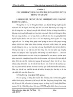
Figure 3.3: 𝑪/𝑵𝟎 of the satellite PRN 09 for the received signal at
every element and beamed signal
Figure 3.3 indicates that the carrier to noise ratio of the signals received
by different elements are different. However, the ratio of the beamed

signal is much higher than that of element.
3.5. Conclusion and discussion
The chapter presented the practical consideration in designing an antenna
array for GNSS application. The result shown in this chapter is a very
promising for not only GNSS application but also the other field.
In the future, we will use such antenna array frontend to suppress
interference, point to the source of the interference and spoofing

17


4. GNSS Snapshot processing techniques for GNSS
receivers
Nowadays, GPS receivers are widely used in many applications ranging
from vehicle navigation to unmanned vehicle guidance, from locationbased services to environment monitoring… The traditional architecture
of GPS receiver has the signal processing part composed of 4 stages:
signal conditioning and digitization, signal synchronization (acquisition,
and tracking), data demodulation, and position-time-velocity calculation
[13]. Among these stages, the most difficult one is the signal
synchronization. This stage is based on the correlation computation
results between the received signal and its local replica to perform signal
acquisition and tracking. However, since the GPS satellites are located
roughly 20,200 km from the Earth, the received signal is very weak even
in open sky environment (nominal C/N0 value of 45dB-Hz). Therefore,
the integration time for each correlation value must be long enough to
achieve a reasonable processing gain so that the signal can appear from
the noise floor (e.g. nominal value being 1ms for coherent integration
time). In harsh environment (under tree, indoor…), the longer coherent
integration time is required. In addition, for PVT computation, a
standalone GPS receiver must be turned on for a minimum 30 seconds to

download a full page of ephemeris data from at least 4 satellites-in-view.
Even an assisted GPS solution, which basically requires a shorter time to
first fix (TTFF), still needs 6 seconds for decoding time stamps for
Position-Velocity-Time (PVT) computation [13].
These lead to the fact that a GPS positioning requires a huge
computational resource, which also implies a huge power consumption.
In recent years, every smartphone has a GPS receiver on it, however, if
the receiver stays on, the battery of the phone will be drained very fast.
Therefore, a more battery capacity is required, however, for devices
which have big concerns on the size and weight (e.g. smartwatches, kid
tracker, pet tracker…), a low power consumption approach is needed for
GPS positioning.

18


Figure 4.1: Snapshot positioning architecture
[14] introduces a technique, namely snapshot positioning. In this
technique, a user is equipped with a GPS data grabber, which collect GPS
signal on site. The dataset is then transmitted to a server (see Figure 4.1).
At the server side, the available GPS data (provided by another GPS
receiver) and the received dataset are used together to compute the
position of the user. In this technique, the most difficult tasks – signal
synchronization and position computation – are performed at the server
side, whereas on the user side, only a simple GPS data grabber with a
communication modem is needed. By this way, the computational
requirement at the user side is relaxed, and eventually, the power
consumption is reduced significantly. Although snapshot receiver was
first proposed by NASA [14] in 1997, it has been widely studied in recent
years due to the increasing demands on low power consumption

positioning for mobile devices, especially for smartwatch, and object
trackers.
In [14], the requirement for using the technique is that we need to know
an approximate position (so-called prior solution), which must be less
than 150 km, equivalent to a half code-length, from the true position.
However, that information is not always available in reality. To overcome
that distance limitation, recent studies, which propose feasible designs of
snapshot receivers for mobile computing [25] [26] use the position of the
base stations of the cellular network as the prior solution. However, due
to the policy of telecommunication companies, that information of base
stations is also not always provided. The work in [3] uses the Doppler
positioning method in order to provide the prior solution for the snapshot
positioning. Although the Doppler positioning is not so precise, however,
that level of accuracy already satisfies the 150-km-requirement. However,
19


the architecture in [15] requires the fine estimation of code delay.
Therefore, the tracking process is mandatory, this leads to power
consumption due to the correlation computation.
Besides the signal processing part which is already relaxed by the
snapshot technique, the communication part needs to control the power
consumption also. Therefore, the size of the dataset must be reduced as
much as possible to meet that requirement. In literature, the GPS data
grabbers use 2 bits for quantization, with the sampling frequency of 2.046
MHz. The sampling frequency has an important impact to the accuracy
of the positioning and cannot be reduced due to the Nyquist criteria.
Meanwhile, the number of quantization bits has impact to the sensitivity
of the positioning, which can be compensated by extending the
integration time. In addition, in the view point of hardware design and

implementation, the 1-bit data stream is much simpler and more stable
than the 2-bit one since the Serial Peripheral Interface (SPI) interface,
which is a fast data transfer protocol, can be used directly in 1-bit stream
to facilitate the data transfer between the frontend and the microprocessor.
This chapter introduces a novel design of low power consumption GPS
positioning solution based on snapshot technique. In this design, a
complete snapshot solution including GPS data grabber, and server
program is presented. The snapshot processing leverages a 1-bit
quantization frontend and the Doppler positioning in order to achieve the
low power consumption objective. The solution is validated with real
GPS signal. The validation results show a 77% reduction in power
consumption in comparison with a typical commercial GPS receiver,
meanwhile the accuracy level is about 14 m in horizontal position, which
can satisfy most of mobile applications.
The remaining part of the chapter is as follows. Section Proposed
Design4.1 presents the architecture of the grabber and the overview of
snapshot technique.
4.1. Proposed Design of GNSS Snapshot Receiver
The proposed design contains 2 parts, namely GPS grabber for collecting
the IF digitalized data and a server software for post-processing to
20


estimate PVT of the GNSS grabber.
4.1.1.

GNSS Grabber

4.2. Server Software
4.3. Loosely coupled Snapshot GNSS/INS

4.4. RESULTS
4.4.1.

Standalone Snapshot GNSS Receiver

Firstly, we evaluate the positioning performance of our solution
with the live-sky signal collected by our GPS grabber. The data
was collected on July, 19th, 2017 at HUST. The configuration of
this experiment is shown.
Due to the similar behaviors of other signals, we shows the acquisition
result of a strong signal (PRN20) and a weak signal (PRN12). As
observed, the peak is emerged from noise floor even this is the weak
signal. The results verify that the solution is able to use in harsh
environments where the GPS signal power is low.
With 10 milliseconds of integration time, 8 satellites in view are acquired.
The code phase, Doppler shift, and Peak to Average Power Ratio (PAPR)
of acquired satellites are represented in the corresponding figure.
Since all measurements show similar behaviors, we take the first
measurement to visualize the work of our proposed solution. To compute
the user position, the Doppler positioning is performed first to produce
the initial solution. As shown in the corresponding figure, the produced
position (blue one) is about 4 km from the user position. This confirms
that the position produced by the Doppler positioning meets the
requirement of a-priori solution for the snapshot positioning (below 150
km from the user position). Using the output from the Doppler
positioning, the solution of the snapshot algorithm is converged after 7
iterations (red ones).
The accuracy of the receiver is shown in the corresponding figure and
Table 3. Clearly, with 14 meters of accuracy, the solution approaches the
accuracy of commercial receivers.

21


Table 3. Positioning Performance of the proposed solution
(100 measurements with the fixed antenna)
𝛿𝐸 (m)
14.12

𝛿𝑁 (m)
14.66

𝛿𝑈 (m)
40.7

𝛿(m)
45.58

Clearly, with 45.58 m of the standard deviation, the accuracy of our
design is better than the previous work (62.81 m) [25]
4.4.2.

Snapshot GNSS/INS Integration

In the second experiment, we benchmark the power consumption of our
solution with Ublox – a low power consumption receiver on the market.
In this experiment, we measure the average current of our grabber with
the various time periods between signal collections. The average power
of our design is inversely propositional to the measurement period while
that of U-blox is unchanged with 22mA in the average chipset. This is
because the grabber lasts 180 milliseconds in one period to collect the

signal nevertheless the update period time and enter the backup mode for
a remaining time.
In our experiments, the chosen IMU sensor and GPS receiver were 3DMGX3 provided by MicroTrain and LEA-6P provided by Ublox,
respectively (Fig. 6). The conducted experiments with two scenarios are
described as below.
In our experiment, the GPS receiver and IMU are all mounted to a fixed
frame and placed on the vehicle. The vehicle is then moved around the
HUST campus following the trajectory illustrated in Fig. 7. In this mode,
the position of every point in the reference trajectory is estimated using
RTK technique. The base station is placed at a reference point in HUST.
We verify the performance of the proposed model in both low DOP and
high DOP cases. Therefore, we decide to choose 4 satellites following
predefined scenarios as follows.
In the first case, the chosen satellites to compute PVT must satisfy the low
DOP (Dilution Of Precision) value criteria (Fig. 8). The experiment lasts
250 seconds.
In the second case, the setup is the same as in the first case except for the
chosen satellites for calculating PVT solution. In this case, the chosen
satellites satisfy the high DOP value criteria (Fig. 10).
22


Conclusion
In this chapter, related theory and implementation of a new design for
energy effective positioning have been presented. The results verify that
the new design can reduce the size of dataset while the overall
performance is higher than previous studies. Moreover, the proposal can
give the position without a-prior knowledge of the initial position.
Future works will focus on improving the accuracy of the solution in
different scenarios.

23


CONCLUSIONS AND FUTURE WORKS
The content of this thesis aims to investigate the potentials and challenges
of modern GNSS receivers under threats. Through the investigation of
properties of modern GNSS receivers, some improvement its
performance is presented. In this thesis, the works devoted to the improve
the modern GNSS receivers are the main contributions, which can be
summarized as follows:
Design and implementation of a software-based GNSS simulator
(Chapter 2): A complete theory and implementation of a GNSS simulator
which is capable of simulating antenna array signals. The block diagrams,
theoretical and practical analyses of all stages in the simulator are
provided especially sampling frequency. The performance evaluation
results prove that the generated signals are reliable to the live sky signals.
Testing with multiple frontends will be the future works of this section.
Antenna array processing for GNSS Receivers (Chapter 3): A technique
for extending the antenna element to infinite theoretically is proposed for
the first time in this thesis. The technique is proved suitable for low-cost
antenna array frontends.
Robust GNSS Snapshot Receiver (Chapter 4): The multi-GNSS snapshot
receiver is proposed. Such receiver is proved that it is suitable for the
discontinuous GNSS signal due to jamming, spoofing or interference

24