Representation learning a review and new perspectives v1

1

Unsupervised Feature Learning and Deep
Learning: A Review and New Perspectives
Yoshua Bengio, Aaron Courville, and Pascal Vincent
Department of computer science and operations research, U. Montreal

arXiv:1206.5538v1 [cs.LG] 24 Jun 2012

✦
Abstract—
The success of machine learning algorithms generally depends on
data representation, and we hypothesize that this is because different representations can entangle and hide more or less the different
explanatory factors of variation behind the data. Although domain
knowledge can be used to help design representations, learning can
also be used, and the quest for AI is motivating the design of more
powerful representation-learning algorithms. This paper reviews recent
work in the area of unsupervised feature learning and deep learning,
covering advances in probabilistic models, manifold learning, and deep
learning. This motivates longer-term unanswered questions about the
appropriate objectives for learning good representations, for computing
representations (i.e., inference), and the geometrical connections between representation learning, density estimation and manifold learning.
Index Terms—Deep learning, feature learning, unsupervised learning,
Boltzmann Machine, RBM, auto-encoder, neural network

1

I NTRODUCTION

Data representation is empirically found to be a core determinant of the performance of most machine learning algorithms.
For that reason, much of the actual effort in deploying machine

learning algorithms goes into the design of feature extraction,
preprocessing and data transformations. Feature engineering
is important but labor-intensive and highlights the weakness
of current learning algorithms, their inability to extract all
of the juice from the data. Feature engineering is a way to
take advantage of human intelligence and prior knowledge to
compensate for that weakness. In order to expand the scope
and ease of applicability of machine learning, it would be
highly desirable to make learning algorithms less dependent
on feature engineering, so that novel applications could be
constructed faster, and more importantly, to make progress
towards Artificial Intelligence (AI). An AI must fundamentally
understand the world around us, and this can be achieved if a
learner can identify and disentangle the underlying explanatory
factors hidden in the observed milieu of low-level sensory data.
When it comes time to achieve state-of-the-art results on
practical real-world problems, feature engineering can be
combined with feature learning, and the simplest way is to
learn higher-level features on top of handcrafted ones. This
paper is about feature learning, or representation learning, i.e.,
learning representations and transformations of the data that
somehow make it easier to extract useful information out of it,
e.g., when building classifiers or other predictors. In the case of
probabilistic models, a good representation is often one that
captures the posterior distribution of underlying explanatory
factors for the observed input.

Among the various ways of learning representations, this
paper also focuses on those that can yield more non-linear,
more abstract representations, i.e. deep learning. A deep

architecture is formed by the composition of multiple levels of
representation, where the number of levels is a free parameter
which can be selected depending on the demands of the given
task. This paper is meant to be a follow-up and a complement
to an earlier survey (Bengio, 2009) (but see also Arel et al.
(2010)). Here we survey recent progress in the area, with an
emphasis on the longer-term unanswered questions raised by
this research, in particular about the appropriate objectives for
learning good representations, for computing representations
(i.e., inference), and the geometrical connections between representation learning, density estimation and manifold learning.
In Bengio and LeCun (2007), we introduce the notion of
AI-tasks, which are challenging for current machine learning
algorithms, and involve complex but highly structured dependencies. For substantial progress on tasks such as computer
vision and natural language understanding, it seems hopeless
to rely only on simple parametric models (such as linear
models) because they cannot capture enough of the complexity
of interest. On the other hand, machine learning researchers
have sought flexibility in local1 non-parametric learners such
as kernel machines with a fixed generic local-response kernel
(such as the Gaussian kernel). Unfortunately, as argued at
length previously (Bengio and Monperrus, 2005; Bengio et al.,
2006a; Bengio and LeCun, 2007; Bengio, 2009; Bengio et al.,
2010), most of these algorithms only exploit the principle
of local generalization, i.e., the assumption that the target
function (to be learned) is smooth enough, so they rely on
examples to explicitly map out the wrinkles of the target
function. Although smoothness can be a useful assumption, it
is insufficient to deal with the curse of dimensionality, because
the number of such wrinkles (ups and downs of the target
function) may grow exponentially with the number of relevant

interacting factors or input dimensions. What we advocate are
learning algorithms that are flexible and non-parametric2 but
do not rely merely on the smoothness assumption. However,
it is useful to apply a linear model or kernel machine on top
1. local in the sense that the value of the learned function at x depends
mostly on training examples x(t) ’s close to x
2. We understand non-parametric as including all learning algorithms
whose capacity can be increased appropriately as the amount of data and its
complexity demands it, e.g. including mixture models and neural networks
where the number of parameters is a data-selected hyper-parameter.


2

of a learned representation: this is equivalent to learning the
kernel, i.e., the feature space. Kernel machines are useful, but
they depend on a prior definition of a suitable similarity metric,
or a feature space in which naive similarity metrics suffice; we
would like to also use the data to discover good features.
This brings us to representation-learning as a core element that can be incorporated in many learning frameworks.
Interesting representations are expressive, meaning that a
reasonably-sized learned representation can capture a huge
number of possible input configurations: that excludes onehot representations, such as the result of traditional clustering algorithms, but could include multi-clustering algorithms
where either several clusterings take place in parallel or the
same clustering is applied on different parts of the input,
such as in the very popular hierarchical feature extraction for
object recognition based on a histogram of cluster categories
detected in different patches of an image (Lazebnik et al.,
2006; Coates and Ng, 2011a). Distributed representations and
sparse representations are the typical ways to achieve such

expressiveness, and both can provide exponential gains over
more local approaches, as argued in section 3.2 (and Figure
3.2) of Bengio (2009). This is because each parameter (e.g.
the parameters of one of the units in a sparse code, or one
of the units in a Restricted Boltzmann Machine) can be reused in many examples that are not simply near neighbors
of each other, whereas with local generalization, different
regions in input space are basically associated with their own
private set of parameters, e.g. as in decision trees, nearestneighbors, Gaussian SVMs, etc. In a distributed representation,
an exponentially large number of possible subsets of features
or hidden units can be activated in response to a given input.
In a single-layer model, each feature is typically associated
with a preferred input direction, corresponding to a hyperplane
in input space, and the code or representation associated
with that input is precisely the pattern of activation (which
features respond to the input, and how much). This is in
contrast with a non-distributed representation such as the
one learned by most clustering algorithms, e.g., k-means,
in which the representation of a given input vector is a
one-hot code (identifying which one of a small number of
cluster centroids best represents the input). The situation seems
slightly better with a decision tree, where each given input is
associated with a one-hot code over the tree leaves, which
deterministically selects associated ancestors (the path from
root to node). Unfortunately, the number of different regions
represented (equal to the number of leaves of the tree) still
only grows linearly with the number of parameters used to
specify it (Bengio and Delalleau, 2011).
The notion of re-use, which explains the power of distributed representations, is also at the heart of the theoretical
advantages behind deep learning, i.e., constructing multiple
levels of representation or learning a hierarchy of features.

The depth of a circuit is the length of the longest path
from an input node of the circuit to an output node of the
circuit. Formally, one can change the depth of a given circuit
by changing the definition of what each node can compute,
but only by a constant factor. The typical computations we
allow in each node include: weighted sum, product, artificial

neuron model (such as a monotone non-linearity on top of an
affine transformation), computation of a kernel, or logic gates.
Theoretical results clearly show families of functions where a
deep representation can be exponentially more efficient than
one that is insufficiently deep (H˚astad, 1986; H˚astad and
Goldmann, 1991; Bengio et al., 2006a; Bengio and LeCun,
2007; Bengio and Delalleau, 2011). If the same family of
functions can be represented with fewer parameters (or more
precisely with a smaller VC-dimension3 ), learning theory
would suggest that it can be learned with fewer examples,
yielding improvements in both computational efficiency and
statistical efficiency.
Another important motivation for feature learning and deep
learning is that they can be done with unlabeled examples,
so long as the factors relevant to the questions we will ask
later (e.g. classes to be predicted) are somehow salient in
the input distribution itself. This is true under the manifold
hypothesis, which states that natural classes and other highlevel concepts in which humans are interested are associated
with low-dimensional regions in input space (manifolds) near
which the distribution concentrates, and that different class
manifolds are well-separated by regions of very low density.
As a consequence, feature learning and deep learning are
intimately related to principles of unsupervised learning, and

they can be exploited in the semi-supervised setting (where
only a few examples are labeled), as well as the transfer
learning and multi-task settings (where we aim to generalize
to new classes or tasks). The underlying hypothesis is that
many of the underlying factors are shared across classes or
tasks. Since representation learning aims to extract and isolate
these factors, representations can be shared across classes and
tasks.
In 2006, a breakthrough in feature learning and deep learning took place (Hinton et al., 2006; Bengio et al., 2007;
Ranzato et al., 2007), which has been extensively reviewed
and discussed in Bengio (2009). A central idea, referred to
as greedy layerwise unsupervised pre-training, was to learn a
hierarchy of features one level at a time, using unsupervised
feature learning to learn a new transformation at each level
to be composed with the previously learned transformations;
essentially, each iteration of unsupervised feature learning adds
one layer of weights to a deep neural network. Finally, the set
of layers could be combined to initialize a deep supervised predictor, such as a neural network classifier, or a deep generative
model, such as a Deep Boltzmann Machine (Salakhutdinov
and Hinton, 2009a).
This paper is about feature learning algorithms that can
be stacked for that purpose, as it was empirically observed
that this layerwise stacking of feature extraction often yielded
better representations, e.g., in terms of classification error (Larochelle et al., 2009b; Erhan et al., 2010b), quality of
the samples generated by a probabilistic model (Salakhutdinov
and Hinton, 2009a) or in terms of the invariance properties of
the learned features (Goodfellow et al., 2009).
Among feature extraction algorithms, Principal Components
3. Note that in our experiments, deep architectures tend to generalize very
well even when they have quite large numbers of parameters.

3

Analysis or PCA (Pearson, 1901; Hotelling, 1933) is probably
the oldest and most widely used. It learns a linear transformation h = f (x) = W T x + b of input x ∈ Rdx , where
the columns of dx × dh matrix W form an orthogonal basis
for the dh orthogonal directions of greatest variance in the
training data. The result is dh features (the components of
representation h) that are decorrelated. Interestingly, PCA
may be reinterpreted from the three different viewpoints from
which recent advances in non-linear feature learning techniques arose: a) it is related to probabilistic models (Section 2)
such as probabilistic PCA, factor analysis and the traditional
multivariate Gaussian distribution (the leading eigenvectors
of the covariance matrix are the principal components); b)
the representation it learns is essentially the same as that
learned by a basic linear auto-encoder (Section 3); and c)
it can be viewed as a simple linear form of manifold learning
(Section 5), i.e., characterizing a lower-dimensional region in
input space near which the data density is peaked. Thus, PCA
may be kept in the back of the reader’s mind as a common
thread relating these various viewpoints. Unfortunately the
expressive power of linear features is very limited: they cannot
be stacked to form deeper, more abstract representations since
the composition of linear operations yields another linear
operation. Here, we focus on recent algorithms that have
been developed to extract non-linear features, which can
be stacked in the construction of deep networks, although
some authors simply insert a non-linearity between learned
single-layer linear projections (Le et al., 2011c; Chen et al.,

2012). Another rich family of feature extraction techniques,
that this review does not cover in any detail due to space
constraints is Independent Component Analysis or ICA (Jutten
and Herault, 1991; Comon, 1994; Bell and Sejnowski, 1997).
Instead, we refer the reader to Hyv¨arinen et al. (2001a);
Hyv¨arinen et al. (2009). Note that, while in the simplest
case (complete, noise-free) ICA yields linear features, in the
more general case it can be equated with a linear generative
model with non-Gaussian independent latent variables, similar
to sparse coding (section 2.1.3), which will yield non-linear
features. Therefore, ICA and its variants like Independent Subspace Analysis (Hyv¨arinen and Hoyer, 2000) and Topographic
ICA (Hyv¨arinen et al., 2001b) can and have been used to build
deep networks (Le et al., 2010, 2011c): see section 8.2. The
notion of obtaining independent components also appears similar to our stated goal of disentangling underlying explanatory
factors through deep networks. However, for complex realworld distributions, it is doubtful that the relationship between
truly independent underlying factors and the observed highdimensional data can be adequately characterized by a linear
transformation.
A novel contribution of this paper is that it proposes
a new probabilistic framework to encompass both traditional, likelihood-based probabilistic models (Section 2) and
reconstruction-based models such as auto-encoder variants
(Section 3). We call this new framework JEPADA, for Joint
Energy in PArameters and DAta: the basic idea is to consider
the training criterion for reconstruction-based models as an
energy function for a joint undirected model linking data and
parameters, with a partition function that marginalizes both.

This paper also raises many questions, discussed but
certainly not completely answered here. What is a good
representation? What are good criteria for learning such
representations? How can we evaluate the quality of a

representation-learning algorithm? Are there probabilistic interpretations of non-probabilistic feature learning algorithms
such as auto-encoder variants and predictive sparse decomposition (Kavukcuoglu et al., 2008), and could we sample
from the corresponding models? What are the advantages
and disadvantages of the probabilistic vs non-probabilistic
feature learning algorithms? Should learned representations
be necessarily low-dimensional (as in Principal Components
Analysis)? Should we map inputs to representations in a
way that takes into account the explaining away effect of
different explanatory factors, at the price of more expensive
computation? Is the added power of stacking representations
into a deep architecture worth the extra effort? What are
the reasons why globally optimizing a deep architecture has
been found difficult? What are the reasons behind the success
of some of the methods that have been proposed to learn
representations, and in particular deep ones?

2

P ROBABILISTIC M ODELS

From the probabilistic modeling perspective, the question of
feature learning can be interpreted as an attempt to recover
a parsimonious set of latent random variables that describe
a distribution over the observed data. We can express any
probabilistic model over the joint space of the latent variables,
h, and observed or visible variables x, (associated with the
data) as p(x, h). Feature values are conceived as the result of
an inference process to determine the probability distribution
of the latent variables given the data, i.e. p(h | x), often
referred to as the posterior probability. Learning is conceived

in term of estimating a set of model parameters that (locally)
maximizes the likelihood of the training data with respect to
the distribution over these latent variables. The probabilistic
graphical model formalism gives us two possible modeling
paradigms in which we can consider the question of inferring
the latent variables: directed and undirected graphical models.
The key distinguishing factor between these paradigms is
the nature of their parametrization of the joint distribution
p(x, h). The choice of directed versus undirected model has
a major impact on the nature and computational costs of the
algorithmic approach to both inference and learning.
2.1

Directed Graphical Models

Directed latent factor models are parametrized through a decomposition of the joint distribution, p(x, h) = p(x | h)p(h),
involving a prior p(h), and a likelihood p(x | h) that
describes the observed data x in terms of the latent factors
h. Unsupervised feature learning models that can be interpreted with this decomposition include: Principal Components
Analysis (PCA) (Roweis, 1997; Tipping and Bishop, 1999),
sparse coding (Olshausen and Field, 1996), sigmoid belief
networks (Neal, 1992) and the newly introduced spike-andslab sparse coding model (Goodfellow et al., 2011).


4

2.1.1

Explaining Away

In the context of latent factor models, the form of the directed
graphical model often leads to one important property, namely
explaining away: a priori independent causes of an event can
become non-independent given the observation of the event.
Latent factor models can generally be interpreted as latent
cause models, where the h activations cause the observed x.
This renders the a priori independent h to be non-independent.
As a consequence recovering the posterior distribution of h:
p(h | x) (which we use as a basis for feature representation)
is often computationally challenging and can be entirely
intractable, especially when h is discrete.
A classic example that illustrates the phenomenon is to
imagine you are on vacation away from home and you receive
a phone call from the company that installed the security
system at your house. They tell you that the alarm has been
activated. You begin worry your home has been burglarized,
but then you hear on the radio that a minor earthquake has
been reported in the area of your home. If you happen to
know from prior experience that earthquakes sometimes cause
your home alarm system to activate, then suddenly you relax,
confident that your home has very likely not been burglarized.
The example illustrates how the observation, alarm activation, rendered two otherwise entirely independent causes,
burglarized and earthquake, to become dependent – in this
case, the dependency is one of mutual exclusivity. Since both
burglarized and earthquake are very rare events and both can
cause alarm activation, the observation of one explains away
the other. The example demonstrates not only how observations can render causes to be statistically dependent, but also
the utility of explaining away. It gives rise to a parsimonious
prediction of the unseen or latent events from the observations.
Returning to latent factor models, despite the computational

obstacles we face when attempting to recover the posterior
over h, explaining away promises to provide a parsimonious
p(h | x) which can be extremely useful characteristic of a
feature encoding scheme.If one thinks of a representation as
being composed of various feature detectors and estimated
attributes of the observed input, it is useful to allow the
different features to compete and collaborate with each other
to explain the input. This is naturally achieved with directed
graphical models, but can also be achieved with undirected
models (see Section 2.2) such as Boltzmann machines if there
are lateral connections between the corresponding units or
corresponding interaction terms in the energy function that
defines the probability model.
2.1.2

Probabilistic Interpretation of PCA

While PCA was not originally cast as probabilistic model, it
possesses a natural probabilistic interpretation (Roweis, 1997;
Tipping and Bishop, 1999) that casts PCA as factor analysis:
p(h)
p(x | h)

=
=

N (0, σh2 I)
N (W h + µx , σx2 I),

(1)

where x ∈ Rdx , h ∈ Rdh and columns of W span the
same space as leading dh principal components, but are not
constrained to be orthonormal.

2.1.3 Sparse Coding
As in the case of PCA, sparse coding has both a probabilistic
and non-probabilistic interpretation. Sparse coding also relates
a latent representation h (either a vector of random variables
or a feature vector, depending on the interpretation) to the
data x through a linear mapping W , which we refer to as the
dictionary. The difference between sparse coding and PCA
is that sparse coding includes a penalty to ensure a sparse
activation of h is used to encode each input x.
Specifically, from a non-probabilistic perspective, sparse
coding can be seen as recovering the code or feature vector
associated to a new input x via:
h∗ = f (x) = argmin x − W h

2
2

+ λ h 1,

(2)

h

Learning the dictionary W can be accomplished by optimizing
the following training criterion with respect to W :

x(t) − W h∗(t)

JSC =

2
2,

(3)

t

where the x(t) is the input vector for example t and h∗(t) are
the corresponding sparse codes determined by Eq. 2. W is
usually constrained to have unit-norm columns (because one
can arbitrarily exchange scaling of column i with scaling of
(t)
hi , such a constraint is necessary for the L1 penalty to have
any effect).
The probabilistic interpretation of sparse coding differs from
that of PCA, in that instead of a Gaussian prior on the latent
random variable h, we use a sparsity inducing Laplace prior
(corresponding to an L1 penalty):
dh

p(h)

λ exp(−λ|hi |)

=
i

p(x | h)

=

N (W h + µx , σx2 I).

(4)

In the case of sparse coding, because we will ultimately
be interested in a sparse representation (i.e. one with many
features set to exactly zero), we will be interested in recovering
the MAP (maximum a posteriori value of h: i.e. h∗ =
argmaxh p(h | x) rather than its expected value Ep(h|x) [h].
Under this interpretation, dictionary learning proceeds as maximizing the likelihood of the data given these MAP values of
h∗ : argmaxW t p(x(t) | h∗(t) ) subject to the norm constraint
on W . Note that this parameter learning scheme, subject to
the MAP values of the latent h, is not standard practice
in the probabilistic graphical model literature. Typically the
likelihood of the data p(x) =
h p(x | h)p(h) is maximized directly. In the presence of latent variables, expectation
maximization (Dempster et al., 1977) is employed where
the parameters are optimized with respect to the marginal
likelihood, i.e., summing or integrating the joint log-likelihood
over the values of the latent variables under their posterior
P (h | x), rather than considering only the MAP values of h.
The theoretical properties of this form of parameter learning
are not yet well understood but seem to work well in practice
(e.g. k-Means vs Gaussian mixture models and Viterbi training
for HMMs). Note also that the interpretation of sparse coding

as a MAP estimation can be questioned (Gribonval, 2011),
because even though the interpretation of the L1 penalty as
a log-prior is a possible interpretation, there can be other
Bayesian interpretations compatible with the training criterion.


5

Sparse coding is an excellent example of the power of
explaining away. The Laplace distribution (equivalently, the
L1 penalty) over the latent h acts to resolve a sparse and
parsimonious representation of the input. Even with a very
overcomplete dictionary with many redundant bases, the MAP
inference process used in sparse coding to find h∗ can pick
out the most appropriate bases and zero the others, despite
them having a high degree of correlation with the input. This
property arises naturally in directed graphical models such as
sparse coding and is entirely owing to the explaining away
effect. It is not seen in commonly used undirected probabilistic
models such as the RBM, nor is it seen in parametric feature
encoding methods such as auto-encoders. The trade-off is
that, compared to methods such as RBMs and auto-encoders,
inference in sparse coding involves an extra inner-loop of
optimization to find h∗ with a corresponding increase in the
computational cost of feature extraction. Compared to autoencoders and RBMs, the code in sparse coding is a free
variable for each example, and in that sense the implicit
encoder is non-parametric.
One might expect that the parsimony of the sparse coding representation and its explaining away effect would be
advantageous and indeed it seems to be the case. Coates
and Ng (2011a) demonstrated with the CIFAR-10 object

classification task (Krizhevsky and Hinton, 2009) with a patchbase feature extraction pipeline, that in the regime with few
(< 1000) labeled training examples per class, the sparse
coding representation significantly outperformed other highly
competitive encoding schemes. Possibly because of these
properties, and because of the very computationally efficient
algorithms that have been proposed for it (in comparison with
the general case of inference in the presence of explaining
away), sparse coding enjoys considerable popularity as a
feature learning and encoding paradigm. There are numerous
examples of its successful application as a feature representation scheme, including natural image modeling (Raina
et al., 2007; Kavukcuoglu et al., 2008; Coates and Ng, 2011a;
Yu et al., 2011), audio classification (Grosse et al., 2007),
natural language processing (Bagnell and Bradley, 2009), as
well as being a very successful model of the early visual
cortex (Olshausen and Field, 1997). Sparsity criteria can also
be generalized successfully to yield groups of features that
prefer to all be zero, but if one or a few of them are active then
the penalty for activating others in the group is small. Different
group sparsity patterns can incorporate different forms of prior
knowledge (Kavukcuoglu et al., 2009; Jenatton et al., 2009;
Bach et al., 2011; Gregor et al., 2011a).

p(hi = 1) = sigmoid(bi ),
−1
),
p(si | hi ) = N (si | hi µi , αii
−1
)
p(xj | s, h) = N (xj | Wj: (h ◦ s), βjj

where sigmoid is the logistic sigmoid function, b is a set
of biases on the spike variables, µ and W govern the linear
dependence of s on h and v on s respectively, α and β are
diagonal precision matrices of their respective conditionals and
h ◦ s denotes the element-wise product of h and s. The state
of a hidden unit is best understood as hi si , that is, the spike
variables gate the slab variables.
The basic form of the S3C model (i.e. a spike-and-slab latent
factor model) has appeared a number of times in different
domains (L¨ucke and Sheikh, 2011; Garrigues and Olshausen,
2008; Mohamed et al., 2011; Titsias and L´azaro-Gredilla,
2011). However, existing inference schemes have at most been
applied to models with hundreds of bases and hundreds of
thousands of examples. Goodfellow et al. (2012) have recently
introduced an approximate variational inference scheme that
scales to the sizes of models and datasets we typically consider
in unsupervised feature learning, i.e. thousands of bases on
millions of examples.
S3C has been applied to the CIFAR-10 and CIFAR-100
object classification tasks (Krizhevsky and Hinton, 2009),
and shows the same pattern as sparse coding of superior
performance in the regime of relatively few (< 1000) labeled
examples per class (Goodfellow et al., 2012). In fact, in both
the CIFAR-100 dataset (with 500 examples per class) and the
CIFAR-10 dataset (when the number of examples is reduced to
a similar range), the S3C representation actually outperforms
sparse coding representations.
2.2 Undirected Graphical Models
Undirected graphical models, also called Markov random
fields, parametrize the joint p(x, h) through a factorization in

terms of unnormalized clique potentials:
p(x, h) =

1
Zθ

ψi (x)
i

Spike-and-Slab Sparse Coding

Spike-and-slab sparse coding (S3C) is a promising example of
a directed graphical model for feature learning (Goodfellow
et al., 2012). The S3C model possesses a set of latent binary
spike variables h ∈ {0, 1}dh , a set of latent real-valued slab
variables s ∈ Rdh , and real-valued dx -dimensional visible vector x ∈ Rdx . Their interaction is specified via the factorization
of the joint p(x, s, h): ∀i ∈ {1, . . . , dh }, j ∈ {1, . . . , dx },

ηj (h)
j

νk (x, h)

(6)

k

where ψi (x), ηj (h) and νk (x, h) are the clique potentials describing the interactions between the visible elements, between
the hidden variables, and those interaction between the visible
and hidden variables respectively. The partition function Zθ

ensures that the distribution is normalized. Within the context
of unsupervised feature learning, we generally see a particular
form of Markov random field called a Boltzmann distribution
with clique potentials constrained to be positive:
p(x, h) =

2.1.4

(5)

1
exp (−Eθ (x, h)) ,
Zθ

(7)

where Eθ (x, h) is the energy function and contains the interactions described by the MRF clique potentials and θ are the
model parameters that characterize these interactions.
A Boltzmann machine is defined as a network of
symmetrically-coupled binary random variables or units.
These stochastic units can be divided into two groups: (1) the
visible units x ∈ {0, 1}dx that represent the data, and (2) the
hidden or latent units h ∈ {0, 1}dh that mediate dependencies


6

between the visible units through their mutual interactions. The
pattern of interaction is specified through the energy function:
EθBM (x, h)

P (x | h) =

P (xj | h)

1
1
= − xT U x − hT V h − xT W h − bT x − dT h, (8)
2
2

where θ = {U, V, W, b, d} are the model parameters
which respectively encode the visible-to-visible interactions, the hidden-to-hidden interactions, the visible-to-hidden
interactions, the visible self-connections, and the hidden
self-connections (also known as biases). To avoid overparametrization, the diagonals of U and V are set to zero.
The Boltzmann machine energy function specifies the probability distribution over the joint space [x, h], via the Boltzmann distribution, Eq. 7, with the partition function Zθ given
by:
···

Zθ =

hd =1

xdx =1 h1 =1

x1 =1

x1 =0

h

exp −EθBM (x, h; θ) .

···
xdx =0 h1 =0

(9)

hd =0
h

This joint probability distribution gives rise to the set of
conditional distributions of the form:




P (hi | x, h\i ) = sigmoid 

Wji xj +
j

Vii hi + di  (10)
i =i





P (xj | h, x\j ) = sigmoid 

Wji xj +
i

Ujj xj + bj  .
j =j

(11)

In general, inference in the Boltzmann machine is intractable.
For example, computing the conditional probability of hi given
the visibles, P (hi | x), requires marginalizing over the rest of
the hiddens which implies evaluating a sum with 2dh −1 terms:
···
h1 =0

hd =1

hi−1 =1 hi+1 =1

h1 =1

P (hi | x) =

h

···
hi−1 =0 hi+1 =0

P (h | x)

(12)

hd =0
h

However with some judicious choices in the pattern of interactions between the visible and hidden units, more tractable
subsets of the model family are possible, as we discuss next.
2.2.1 Restricted Boltzmann Machines
The restricted Boltzmann machine (RBM) is likely the most
popular subclass of Boltzmann machine. It is defined by
restricting the interactions in the Boltzmann energy function,
in Eq. 8, to only those between h and x, i.e. EθRBM is EθBM with
U = 0 and V = 0. As such, the RBM can be said to form a
bipartite graph with the visibles and the hiddens forming two
layers of vertices in the graph (and no connection between
units of the same layer). With this restriction, the RBM
possesses the useful property that the conditional distribution
over the hidden units factorizes given the visibles:
P (h | x) =

j

P (xj = 1 | h) = sigmoid

i

2.3 RBM parameter estimation
In this section we discuss several algorithms for training
the restricted Boltzmann machine. Many of the methods we

discuss are applicable to more general undirected graphical
models, but are particularly practical in the RBM setting.
As discussed in Sec. 2.1, in training probabilistic models
parameters are typically adapted in order to maximize the likelihood of the training data (or equivalently the log-likelihood,
or its penalized version which adds a regularization term).
With T training examples, the log likelihood is given by:
T

T

log P (x(t) ; θ) =
t=1

P (x(t) , h; θ).

log
t=1

Wji xj + di

(13)

j

Likewise, the conditional distribution over the visible units
given the hiddens also factorizes:

(15)

h∈{0,1}dh

One straightforward way we can consider maximizing this
quantity is to take small steps uphill, following the loglikelihood gradient, to find a local maximum of the likelihood.
For any Boltzmann machine, the gradient of the log-likelihood
of the data is given by:
T

T

log p(x(t) )

=

−

t=1

Ep(h|x(t) )
t=1
T

P (hi = 1 | x) = sigmoid

(14)

This conditional factorization property of the RBM immediately implies that most inferences we would like make are
readily tractable. For example, the RBM feature representation
is taken to be the set of posterior marginals P (hi | x) which
are, given the conditional independence described in Eq. 13,
are immediately available. Note that this is in stark contrast

to the situation with popular directed graphical models for
unsupervised feature extraction, where computing the posterior
probability is intractable.
Importantly, the tractability of the RBM does not extend to
its partition function, which still involves sums with exponential number of terms. It does imply however that we can limit
the number of terms to min{2dx , 2dh }. Usually this is still an
unmanageable number of terms and therefore we must resort
to approximate methods to deal with its estimation.
It is difficult to overstate the impact the RBM has had to
the fields of unsupervised feature learning and deep learning.
It has been used in a truly impressive variety of applications, including fMRI image classification (Schmah et al.,
2009), motion and spatial transformations (Taylor and Hinton,
2009; Memisevic and Hinton, 2010), collaborative filtering
(Salakhutdinov et al., 2007) and natural image modeling
(Ranzato and Hinton, 2010; Courville et al., 2011b). In the
next section we review the most popular methods for training
RBMs.

∂
∂θi

P (hi | x)

Wji hi + bj
i

+

Ep(x,h)
t=1

∂ RBM (t)
Eθ
(x , h)
∂θi

∂ RBM
Eθ
(x, h) , (16)
∂θi

where we have the expectations with respect to p(h(t) | x(t) )
in the “clamped” condition (also called the positive phase),


7

and over the full joint p(x, h) in the “unclamped” condition
(also called the negative phase). Intuitively, the gradient acts
to locally move the model distribution (the negative phase
distribution) toward the data distribution (positive phase distribution), by pushing down the energy of (h, x(t) ) pairs (for
h ∼ P (h|x(t) )) while pushing up the energy of (h, x) pairs
(for (h, x) ∼ P (h, x)) until the two forces are in equilibrium.
The RBM conditional independence properties imply that
the expectation in the positive phase of Eq. 16 is readily
tractable. The negative phase term – arising from the partition
function’s contribution to the log-likelihood gradient – is more
problematic because the computation of the expectation over
the joint is not tractable. The various ways of dealing with the
partition function’s contribution to the gradient have brought

about a number of different training algorithms, many trying
to approximate the log-likelihood gradient.
To approximate the expectation of the joint distribution in
the negative phase contribution to the gradient, it is natural to
again consider exploiting the conditional independence of the
RBM in order to specify a Monte Carlo approximation of the
expectation over the joint:
Ep(x,h)

1
∂ RBM
Eθ
(x, h) ≈
∂θi
L

L

l=1

∂ RBM (l) ˜ (l)
Eθ
(˜
x , h ),
∂θi

(17)

with the samples drawn by a block Gibbs MCMC (Markov
chain Monte Carlo) sampling scheme from the model distribution:

x
˜(l)
˜ (l)
h

∼

˜ (l−1) )
P (x | h

∼

P (h | x
˜(l) ).

Naively, for each gradient update step, one would start a
Gibbs sampling chain, wait until the chain converges to the
equilibrium distribution and then draw a sufficient number of
samples to approximate the expected gradient with respect
to the model (joint) distribution in Eq. 17. Then restart the
process for the next step of approximate gradient ascent on
the log-likelihood. This procedure has the obvious flaw that
waiting for the Gibbs chain to “burn-in” and reach equilibrium
anew for each gradient update cannot form the basis of a practical training algorithm. Contrastive divergence (Hinton, 1999;
Hinton et al., 2006), stochastic maximum likelihood (Younes,
1999; Tieleman, 2008) and fast-weights persistent contrastive
divergence or FPCD (Tieleman and Hinton, 2009) are all
examples of algorithms that attempt sidestep the need to burnin the negative phase Markov chain.
2.3.1 Contrastive Divergence:
Contrastive divergence (CD) estimation (Hinton, 1999; Hinton

et al., 2006) uses a biased estimate of the gradient in Eq. 16
by approximating the negative phase expectation with a very
short Gibbs chain (often just one step) initialized at the
training data used in the positive phase. This initialization
is chosen to reduce the variance of the negative expectation
based on samples from the short running Gibbs sampler. The
intuition is that, while the samples drawn from very short
Gibbs chains may be a heavily biased (and poor) representation of the model distribution, they are at least moving in
the direction of the model distribution relative to the data

distribution represented by the positive phase training data.
Consequently, they may combine to produce a good estimate
of the gradient, or direction of progress. Much has been written
about the properties and alternative interpretations of CD, e.g.
Carreira-Perpi˜nan and Hinton (2005); Yuille (2005); Bengio
and Delalleau (2009); Sutskever and Tieleman (2010).
2.3.2 Stochastic Maximum Likelihood:
The stochastic maximum likelihood (SML) algorithm (also
known as persistent contrastive divergence or PCD) (Younes,
1999; Tieleman, 2008) is an alternative way to sidestep an
extended burn-in of the negative phase Gibbs sampler. At each
gradient update, rather than initializing the Gibbs chain at the
positive phase sample as in CD, SML initializes the chain at
the last state of the chain used for the previous update. In
other words, SML uses a continually running Gibbs chain (or
often a number of Gibbs chains run in parallel) from which
samples are drawn to estimate the negative phase expectation.
Despite the model parameters changing between updates, these
changes should be small enough that only a few steps of Gibbs
(in practice, often one step is used) are required to maintain

samples from the equilibrium distribution of the Gibbs chain,
i.e. the model distribution.
One aspect of SML that has received considerable recent
attention is that it relies on the Gibbs chain to have reasonably
good mixing properties for learning to succeed. Typically, as
learning progresses and the weights of the RBM grow, the
ergodicity of the Gibbs sample begins to break down. If the
learning rate associated with gradient ascent θ ← θ + gˆ
(with E[ˆ
g ] ≈ ∂ log∂θpθ (x) ) is not reduced to compensate, then
the Gibbs sampler will diverge from the model distribution
and learning will fail. There have been a number of attempts
made to address the failure of Gibbs chain mixing in the
context of SML. Desjardins et al. (2010); Cho et al. (2010);
Salakhutdinov (2010b,a) have all considered various forms of
tempered transitions to improve the mixing rate of the negative
phase Gibbs chain.
Tieleman and Hinton (2009) have proposed quite a different approach to addressing potential mixing problems of
SML with their fast-weights persistent contrastive divergence
(FPCD), and it has also been exploited to train Deep Boltzmann Machines (Salakhutdinov, 2010a) and construct a pure
sampling algorithm for RBMs (Breuleux et al., 2011). FPCD
builds on the surprising but robust tendency of Gibbs chains
to mix better during SML learning than when the model
parameters are fixed. The phenomena is rooted in the form of
the likelihood gradient itself (Eq. 16). The samples drawn from
the SML Gibbs chain are used in the negative phase of the
gradient, which implies that the learning update will slightly
increase the energy (decrease the probability) of those samples,
making the region in the neighborhood of those samples
less likely to be resampled and therefore making it more

likely that the samples will move somewhere else (typically
going near another mode). Rather than drawing samples from
the distribution of the current model (with parameters θ),
FPCD exaggerates this effect by drawing samples from a local
perturbation of the model with parameters θ∗ and an update
specified by:


8

∗
θt+1
= (1 − η)θt+1 + ηθt∗ +

∗

∂
∂θi

T

log p(x(t) ) ,

(18)

t=1

where ∗ is the relatively large fast-weight learning rate
( ∗ > ) and 0 < η < 1 (but near 1) is a forgetting factor
that keeps the perturbed model close to the current model.

Unlike tempering, FPCD does not converge to the model
distribution as and ∗ go to 0, and further work is necessary
to characterize the nature of its approximation to the model
distribution. Nevertheless, FPCD is a popular and apparently
effective means of drawing approximate samples from the
model distribution that faithfully represent its diversity, at the
price of sometimes generating spurious samples in between
two modes (because the fast weights roughly correspond to
a smoothed view of the current model’s energy function). It
has been applied in a variety of applications (Tieleman and
Hinton, 2009; Ranzato et al., 2011; Kivinen and Williams,
2012) and it has been transformed into a pure sampling
algorithm (Breuleux et al., 2011) that also shares this fast
mixing property with herding (Welling, 2009), for the same
reason.
2.3.3 Pseudolikelihood and Ratio-matching
While CD, SML and FPCD are by far the most popular methods for training RBMs and RBM-based models, all of these
methods are perhaps most naturally described as offering different approximations to maximum likelihood training. There
exist other inductive principles that are alternatives to maximum likelihood that can also be used to train RBMs. In particular, these include pseudo-likelihood (Besag, 1975) and ratiomatching (Hyv¨arinen, 2007). Both of these inductive principles
attempt to avoid explicitly dealing with the partition function,
and their asymptotic efficiency has been analyzed (Marlin and
de Freitas, 2011). Pseudo-likelihood seeks to maximize the
product of all one-dimensional conditional distributions of the
form P (xd |x\d ), while ratio-matching can be interpreted as an
extension of score matching (Hyv¨arinen, 2005) to discrete data
types. Both methods amount to weighted differences of the
gradient of the RBM free energy4 evaluated at a data point and
at all neighboring points within a hamming ball of radius 1.
One drawback of these methods is that the computation of the
statistics for all neighbors of each training data point require a

significant computational overhead that scales linearly with the
dimensionality of the input, nd . CD, SML and FPCD have no
such issue. Marlin et al. (2010) provides an excellent survey
of these methods and their relation to CD and SML. They
also empirically compared all of these methods on a range of
classification, reconstruction and density modeling tasks and
found that, in general, SML provided the best combination of
overall performance and computational tractability. However,
in a later study, the same authors (Swersky et al., 2011)
found denoising score matching (Kingma and LeCun, 2010;
Vincent, 2011) to be a competitive inductive principle both
in terms of classification performance (with respect to SML)
4. The free energy F (x; θ) is defined in relation to the marginal likelihood
of the data: F (x; θ) = − log P (x) − log Zθ and in the case of the RBM is
tractable.

and in terms of computational efficiency (with respect to
analytically obtained score matching). Note that denoising
score matching is a special case of the denoising auto-encoder
training criterion (Section 3.3) when the reconstruction error
residual equals a gradient, i.e., the score function associated
with an energy function, as shown in (Vincent, 2011).
2.4 Models with Non-Diagonal Conditional Covariance
One of the most popular domains of application of unsupervised feature learning methods are vision tasks, where we seek
to learn basic building blocks for images and videos which are
usually represented by vectors of reals, i.e. x ∈ Rdx .
The Inductive Bias of the Gaussian RBM
The most straightforward approach – and until recently the
most popular – to modeling this kind of real-valued observations within the RBM framework has been the so-called
Gaussian RBM. With the number of hidden units dh = Nm ,

hm ∈ {0, 1}Nm and x ∈ Rdx , the Gaussian RBM model is
specified by the energy function:
Eθm (x, hm )

1
= x·x−
2

Nm

Nm

x·

Wi hm
i

m
bm
i · hi ,

−

i=1

(19)

i=1

where Wi is the weight vector associated with hidden unit hm

i
and bm is a vector of biases.
The Gaussian RBM is defined such that the conditional
distribution of the visible layer given the hidden layer is a fixed
covariance Gaussian with the conditional mean parametrized
by the product of a weight matrix and a binary hidden vector:
p(x | h) = N (W h, σI)

(20)

Thus, in considering the marginal p(x) = h p(x | h)p(h),
the Gaussian RBM can be interpreted as a Gaussian mixture
model with each setting of the hidden units specifying the
position of a mixture component. While the number of mixture
components is potentially very large, growing exponentially in
the number of hidden units, capacity is controlled by these
mixture components sharing a relatively small number of
parameters.
The GRBM has proved somewhat unsatisfactory as a model
of natural images, as the trained features typically do not
represent sharp edges that occur at object boundaries and lead
to latent representations that are not particularly useful features
for classification tasks (Ranzato and Hinton, 2010). Ranzato
and Hinton (2010) argue that the failure of the GRBM to adequately capture the statistical structure of natural images stems
from the exclusive use of the model capacity to capture the
conditional mean at the expense of the conditional covariance.
Natural images, they argue, are chiefly characterized by the
covariance of the pixel values not by their absolute values.
This point is supported by the common use of preprocessing
methods that standardize the global scaling of the pixel values

across images in a dataset or across the pixel values within
each image.
In the remainder of this section we discuss a few alternative
models that each attempt to take on this objective of better
modeling conditional covariances. As a group, these methods


9

constitute a significant step forward in our efforts in learning
useful features of natural image data and other real-valued
data.
2.4.1 The Mean and Covariance RBM
One recently introduced approach to modeling real-valued data
is the mean and covariance RBM (mcRBM) (Ranzato and Hinton, 2010). Like the Gaussian RBM, the mcRBM is a 2-layer
Boltzmann machine that explicitly models the visible units as
Gaussian distributed quantities. However unlike the Gaussian
RBM, the mcRBM uses its hidden layer to independently
parametrize both the mean and covariance of the data through
two sets of hidden units. The mcRBM is a combination
of the covariance RBM (cRBM) (Ranzato et al., 2010a),
that models the conditional covariance, with the Gaussian
RBM that captures the conditional mean. Specifically, with
Nc covariance hidden units, hc ∈ {0, 1}Nc , and Nm mean
hidden units, hm ∈ {0, 1}Nm and, as always, taking the
dimensionality of the visible units to be dx , x ∈ Rdx , the
mcRBM model with dh = Nm + Nc hidden units is defined
via the energy function5 :
1
Eθ (x, h , h ) = −

2
c

Nc Nc

2

hcj xT Cj

m

j=1 j=1

Nc

bcj hci + Eθm (x, hm ),

−

(21)

j=1

where Cj is the weight vector associated with covariance unit
hci and bc is a vector of covariance unit biases. This energy
function gives rise to a set of conditional distributions over
the visible and hidden units. In particular, as desired, the
conditional distribution over the visible units given the mean
and covariance hidden units is a fully general multivariate
Gaussian distribution:

Nm
p(x | hm , hc ) = N

Wj hm

Σ

,Σ ,

(22)

j=1

−1

Nc

T
. The
with covariance matrix Σ =
j=1 hj Cj Cj + I
m
conditional distributions over the binary hidden units hi and
hci form the basis for the feature representation in the mcRBM
and are given by:
Nm

P (hm
i = 1 | x)

=

Wi hci − bm
i

sigmoid

,

i=1

P (hcj = 1 | x)

=

sigmoid

1
2

Nc

hcj xT Cj

2

− bcj

,

j=1

(23)

Like other RBM-based models, the mcRBM can be trained
using either CD or SML (Ranzato and Hinton, 2010). There is,
however, one significant difference: due to the covariance contributions to the conditional Gaussian distribution in Eq. 22,
the sampling from this conditional, which is required as part
of both CD and SML would require computing the inverse
in the expression for Σ at every iteration of learning. With
5. In the interest of simplicity we have suppressed some details of the
mcRBM energy function, please refer to the original exposition in Ranzato
and Hinton (2010).

even a moderately large input dimension dx , this leads to
an impractical computational burden. The solution adopted by
Ranzato and Hinton (2010) is to avoid direct sampling from
the conditional 22 by using hybrid Monte Carlo (Neal, 1993)
to draw samples from the marginal p(x) via the mcRBM free
energy.
As a model of real-valued data, the mcRBM has shown
considerable potential. It has been used in an object classification in natural images (Ranzato and Hinton, 2010) as well as
the basis of a highly successful phoneme recognition system
(Dahl et al., 2010) whose performance surpassed the previous
state-of-the-art in this domain by a significant margin. Despite
these successes, it seems that due to difficulties in training the
mcRBM, the model is presently being superseded by the mPoT
model. We discuss this model next.
2.4.2 Mean - Product of Student’s T-distributions
The product of Student’s T-distributions model (Welling et al.,

2003) is an energy-based model where the conditional distribution over the visible units conditioned on the hidden variables is a multivariate Gaussian (non-diagonal covariance) and
the complementary conditional distribution over the hidden
variables given the visibles are a set of independent Gamma
distributions. The PoT model has recently been generalized to
the mPoT model (Ranzato et al., 2010b) to include nonzero
Gaussian means by the addition of Gaussian RBM-like hidden
units, similarly to how the mcRBM generalizes the cRBM.
Using the same notation as we did when we described the
mcRBM above, the mPoT energy function is given as:
EθmPoT (x, hm , hc ) =
hcj 1 +
j

1
CjT x
2

2

+ (1 − γj ) log hcj

+ Eθm (x, hm )

(24)

where, as in the case of the mcRBM, Cj is the weight vector
associated with covariance unit hcj . Also like the mcRBM,
the mPoT model energy function specifies a fully general
multivariate Gaussian conditional distribution over the inputs
given in Eq 22. However, unlike in the mcRBM, the hidden

covariance units are positive, real-valued (hc ∈ R+ ), and
conditionally Gamma-distributed:
p(hcj | x) = G γj , 1 +

1
CjT x
2

2

(25)

Thus, the mPoT model characterizes the covariance of realvalued inputs with real-valued Gamma-distributed hidden
units.
Since the PoT model gives rise to nearly the identical
multivariate Gaussian conditional distribution over the input as
the mcRBM, estimating the parameters of the mPoT model encounters the same difficulties as encountered with the mcRBM.
The solution is the same: direct sampling of p(x) via hybrid
Monte Carlo.
The mPoT model has been used to synthesize large-scale
natural images (Ranzato et al., 2010b) that show large-scale
features and shadowing structure. It has been used to model
natural textures (Kivinen and Williams, 2012) in a tiledconvolution configuration (see section 8.2) and has also been
used to achieve state-of-the-art performance on a facial expression recognition task (Ranzato et al., 2011).


10

2.4.3 The Spike-and-Slab RBM
Another recently introduced RBM-based model with the objective of having the hidden units encode both the mean

and covariance information is the spike-and-slab Restricted
Boltzmann Machine (ssRBM) (Courville et al., 2011a,b). The
ssRBM is defined as having both a real-valued “slab” variable
and a binary “spike” variable associated with each unit in the
hidden layer. In structure, it can be thought of as augmenting
each hidden unit of the standard Gaussian RBM with a realvalued variable.
More specifically, the i-th hidden unit (where 1 ≤ i ≤ dh )
is associated with a binary spike variable: hi ∈ {0, 1} and a
real-valued variable6 si ∈ R. The ssRBM energy function is
given as:
dh

xT Wi si hi +

Eθ (x, s, h) = −
i=1

1
+
2

dh

dh

αi s2i −
i=1

1 T
x Λx

2
dh

αi µi si hi −
i=1

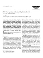
images and has performed well in the role (Courville et al.,
2011a,b). When trained convolutionally (see Section 8.2) on
full CIFAR-10 natural images, the model demonstrated the
ability to generate natural image samples that seem to capture
the broad statistical structure of natural images, as illustrated
with the samples of Figure 1.

dh

αi µ2i hi ,

b i hi +
i=1

(26)

i=1

where Wi refers to the ith weight matrix of size dx × dh , the
bi are the biases associated with each of the spike variables hi ,
and αi and Λ are diagonal matrices that penalize large values
of si 22 and v 22 respectively.
The distribution p(x | h) is determined by analytically
marginalizing over the s variables.

dh

p(x | h) = N

Wi µi hi , Covx|h

Covv|h

(27)

i=1
−1

h
αi−1 hi Wi WiT
, the last equality
where Covx|h = Λ − di=1
holds only if the covariance matrix Covx|h is positive definite.
Strategies for ensuring positive definite Covx|h are discussed
in Courville et al. (2011b). Like the mcRBM and the mPoT
model, the ssRBM gives rise to a fully general multivariate
Gaussian conditional distribution p(x | h).
Crucially, the ssRBM has the property that while the conditional p(x | h) does not easily factor, all the other relevant
conditionals do, with components given by:

αi−1 xT Wi + µi hi , αi−1 ,

p(si | x, h)

=

N

p(hi = 1 | x)

=

sigmoid

p(x | s, h)

=

N

1 −1 T
α (x Wi )2 + xT Wi µi + bi ,
2 i
dh

Λ−1

Wi si hi , Λ−1
i=1

In training the ssRBM, these factored conditionals are exploited to use a 3-phase block Gibbs sampler as an inner loop
to either CD or SML. Thus unlike the mcRBM or the mPoT
alternatives, the ssRBM can make use of efficient and simple
Gibbs sampling during training and inference, and does not
need to resort to hybrid Monte Carlo (which has extra hyperparameters).

The ssRBM has been demonstrated as a feature learning
and extraction scheme in the context of CIFAR-10 object
classification (Krizhevsky and Hinton, 2009) from natural
6. The ssRBM can be easily generalized to having a vector of slab variables
associated with each spike variable(Courville et al., 2011a). For simplicity of
exposition we will assume a scalar si .

Fig. 1. (Top) Samples from a convolutionally trained µ-ssRBM,
see details in Courville et al. (2011b). (Bottom) The images in
the CIFAR-10 training set closest (L2 distance with contrast normalized training images) to the corresponding model samples.
The model does not appear to be capturing the natural image
statistical structure by overfitting particular examples from the
dataset.

2.4.4 Comparing the mcRBM, mPoT and ssRBM
The mcRBM, mPoT and ssRBM each set out to model
real-valued data such that the hidden units encode not only
the conditional mean of the data but also its conditional
covariance. The most obvious difference between these models
is the natural of the sampling scheme used in training them.
As previously discussed, while both the mcRBM and mPoT
models resort to hybrid Monte Carlo, the design of the ssRBM
admits a simple and efficient Gibbs sampling scheme. It
remains to be determined if this difference impacts the relative
feasibility of the models.
A somewhat more subtle difference between these models is
how they encode their conditional covariance. Despite significant differences in the expression of their energy functions,
the mcRBM and the mPoT (Eq. 21 versus Eq. 24), they
are very similar in how they model the covariance structure
of the data, in both cases conditional covariance is given

−1

Nc

c
T
by
. Both models use the activation
j=1 hj Cj Cj + I
of the hidden units hj > 0 to enforces constraints on the
covariance of x, in the direction of Cj . The ssRBM, on the
other hand, specifies the conditional covariance of p(x | h)

as

Λ−

dh
i=1

αi−1 hi Wi WiT

−1

and uses the hidden spike


11

activations hi = 1 to pinch the precision matrix along the

direction specified by the corresponding weight vector.
In the complete case, when the dimensionality of the hidden
layer equals that of the input, these two ways to specify the
conditional covariance are roughly equivalent. However, they
diverge when the dimensionality of the hidden layer is significantly different from that of the input. In the over-complete
setting, sparse activation with the ssRBM parametrization
permits significant variance (above the nominal variance given
by Λ−1 ) only in the select directions of the sparsely activated
hi . This is a property the ssRBM shares with sparse coding
models (Olshausen and Field, 1997; Grosse et al., 2007) where
the sparse latent representation also encodes directions of
variance above a nominal value. In the case of the mPoT
or mcRBM, an over-complete set of constraints on the covariance implies that capturing arbitrary covariance along a
particular direction of the input requires decreasing potentially
all constraints with positive projection in that direction. This
perspective would suggest that the mPoT and mcRBM do not
appear to be well suited to provide a sparse representation in
the overcomplete setting.

3

R EGULARIZED AUTO -E NCODERS

Within the framework of probabilistic models adopted in
Section 2, features are always associated with latent variables,
specifically with their posterior distribution given an observed
input x. Unfortunately this posterior distribution tends to
become very complicated and intractable if the model has
more than a couple of interconnected layers, whether in
the directed or undirected graphical model frameworks. It

then becomes necessary to resort to sampling or approximate
inference techniques, and to pay the associated computational
and approximation error price. This is in addition to the difficulties raised by the intractable partition function in undirected
graphical models. Moreover a posterior distribution over latent
variables is not yet a simple usable feature vector that can
for example be fed to a classifier. So actual feature values
are typically derived from that distribution, taking the latent
variable’s expectation (as is typically done with RBMs) or
finding their most likely value (as in sparse coding). If we
are to extract stable deterministic numerical feature values in
the end anyway, an alternative (apparently) non-probabilistic
feature learning paradigm that focuses on carrying out this part
of the computation, very efficiently, is that of auto-encoders.
3.1 Auto-Encoders
In the auto-encoder framework (LeCun, 1987; Hinton and
Zemel, 1994), one starts by explicitly defining a featureextracting function in a specific parametrized closed form. This
function, that we will denote fθ , is called the encoder and
will allow the straightforward and efficient computation of a
feature vector h = fθ (x) from an input x. For each example
x(t) from a data set {x(1) , . . . , x(T ) }, we define
h(t) = fθ (x(t) )
(t)

(28)

where h is the feature-vector or representation or code computed from x(t) . Another closed form parametrized function
gθ , called the decoder, maps from feature space back into

input space, producing a reconstruction r = gθ (h). The
set of parameters θ of the encoder and decoder are learned

simultaneously on the task of reconstructing as best as possible
the original input, i.e. attempting to incur the lowest possible
reconstruction error L(x, r) – a measure of the discrepancy
between x and its reconstruction – on average over a training
set.
In summary, basic auto-encoder training consists in finding
a value of parameter vector θ minimizing reconstruction error
JDAE (θ)

L(x(t) , gθ (fθ (x(t) ))).

=

(29)

t

This minimization is usually carried out by stochastic gradient
descent as in the training of Multi-Layer-Perceptrons (MLPs).
Since auto-encoders were primarily developed as MLPs predicting their input, the most commonly used forms for the
encoder and decoder are affine mappings, optionally followed
by a non-linearity:
fθ (x)
gθ (h)

=
=

sf (b + W x)
sg (d + W h)

(30)
(31)

where sf and sg are the encoder and decoder activation
functions (typically the element-wise sigmoid or hyperbolic
tangent non-linearity, or the identity function if staying linear).
The set of parameters of such a model is θ = {W, b, W , d}
where b and d are called encoder and decoder bias vectors,
and W and W are the encoder and decoder weight matrices.
The choice of sg and L depends largely on the input domain
range. A natural choice for an unbounded domain is a linear
decoder with a squared reconstruction error, i.e. sg (a) = a and
L(x, r) = x − r 2 . If inputs are bounded between 0 and 1
however, ensuring a similarly-bounded reconstruction can be
achieved by using sg = sigmoid. In addition if the inputs are
of a binary nature, a binary cross-entropy loss7 is sometimes
used.
In the case of a linear auto-encoder (linear encoder and
decoder) with squared reconstruction error, the basic autoencoder objective in Equation 29 is known to learn the same
subspace8 as PCA. This is also true when using a sigmoid
nonlinearity in the encoder (Bourlard and Kamp, 1988), but
not if the weights W and W are tied (W = W T ).
Similarly, Le et al. (2011b) recently showed that adding a
regularization term of the form i j s3 (Wj xi ) to a linear
auto-encoder with tied weights, where s3 is a nonlinear convex
function, yields an efficient algorithm for learning linear ICA.
If both encoder and decoder use a sigmoid non-linearity,
then fθ (x) and gθ (h) have the exact same form as the conditionals P (h | v) and P (v | h) of binary RBMs (see Section
2.2.1). This similarity motivated an initial study (Bengio et al.,

2007) of the possibility of replacing RBMs with auto-encoders
as the basic pre-training strategy for building deep networks,
as well as the comparative analysis of auto-encoder reconstruction error gradient and contrastive divergence updates (Bengio
and Delalleau, 2009).
x
7. L(x, r) = − di=1
xi log(ri ) + (1 − ri ) log(1 − ri )
8. Contrary to traditional PCA loading factors, but similarly to the parameters learned by probabilistic PCA, the weight vectors learned by such an
auto-encoder are not constrained to form an orthonormal basis, nor to have a
meaningful ordering. They will however span the same subspace.


12

One notable difference in the parametrization is that RBMs
use a single weight matrix, which follows naturally from their
energy function, whereas the auto-encoder framework allows
for a different matrix in the encoder and decoder. In practice
however, weight-tying in which one defines W = W T may
be (and is most often) used, rendering the parametrizations
identical. The usual training procedures however differ greatly
between the two approaches. A practical advantage of training
auto-encoder variants is that they define a simple tractable
optimization objective that can be used to monitor progress.
Traditionally, auto-encoders, like PCA, were primarily seen
as a dimensionality reduction technique and thus used a
bottleneck, i.e. dh < dx . But successful uses of sparse coding
and RBM approaches tend to favor learning over-complete
representations, i.e. dh > dx . This can render the autoencoding problem too simple (e.g. simply duplicating the input
in the features may allow perfect reconstruction without having

extracted any more meaningful feature). Thus alternative ways
to “constrain” the representation, other than constraining its
dimensionality, have been investigated. We broadly refer to
these alternatives as “regularized” auto-encoders. The effect
of a bottleneck or of these regularization terms is that the
auto-encoder cannot reconstruct well everything, it is trained
to reconstruct well the training examples and generalization
means that reconstruction error is also small on test examples.
An interesting justification (Ranzato et al., 2008) for the
sparsity penalty (or any penalty that restricts in a soft way
the volume of hidden configurations easily accessible by the
learner) is that it acts in spirit like the partition function of
RBMs, by making sure that only few input configurations can
have a low reconstruction error. See Section 4 for a longer
discussion on the lack of partition function in auto-encoder
training criteria.
3.2 Sparse Auto-Encoders
The earliest use of single-layer auto-encoders for building
deep architectures by stacking them (Bengio et al., 2007)
considered the idea of tying the encoder weights and decoder
weights to restrict capacity as well as the idea of introducing
a form of sparsity regularization (Ranzato et al., 2007).
Several ways of introducing sparsity in the representation
learned by auto-encoders have then been proposed, some by
penalizing the hidden unit biases (making these additive offset
parameters more negative) (Ranzato et al., 2007; Lee et al.,
2008; Goodfellow et al., 2009; Larochelle and Bengio, 2008)
and some by directly penalizing the output of the hidden unit
activations (making them closer to their saturating value at
0) (Ranzato et al., 2008; Le et al., 2011a; Zou et al., 2011).

Note that penalizing the bias runs the danger that the weights
could compensate for the bias, which could hurt the numerical
optimization of parameters. When directly penalizing the
hidden unit outputs, several variants can be found in the
literature, but no clear comparative analysis has been published
to evaluate which one works better. Although the L1 penalty
(i.e., simply the sum of output elements hj in the case of
sigmoid non-linearity) would seem the most natural (because
of its use in sparse coding), it is used in few papers involving
sparse auto-encoders. A close cousin of the L1 penalty is the

Student-t penalty (log(1 + h2j )), originally proposed for sparse
coding (Olshausen and Field, 1997). Several papers penalize
¯ j (e.g. over a minibatch), and instead
the average output h
of pushing it to 0, encourage it to approach a fixed target,
either through a mean-square error penalty, or maybe more
ˆ behaves like a probability), a Kullbacksensibly (because h
Liebler divergence with respect to the binomial distribution
¯ j − (1 − ρ) log(1 − h
¯ j )+constant,
with probability ρ, −ρ log h
e.g., with ρ = 0.05.
3.3 Denoising Auto-Encoders
Vincent et al. (2008, 2010) proposed altering the training
objective in Equation 29 from mere reconstruction to that
of denoising an artificially corrupted input, i.e. learning to
reconstruct the clean input from a corrupted version. Learning
the identity is no longer enough: the learner must capture the
structure of the input distribution in order to optimally undo

the effect of the corruption process, with the reconstruction
essentially being a nearby but higher density point than the
corrupted input.
Formally, the objective optimized by such a Denoising
Auto-Encoder (DAE) is:
JDAE

x)))
Eq(˜x|x(t) ) L(x(t) , gθ (fθ (˜

=

(32)

t

where Eq(˜x|x(t) ) [·] denotes the expectation over corrupted examples x
˜ drawn from corruption process q(˜
x|x(t) ). In practice
this is optimized by stochastic gradient descent, where the
stochastic gradient is estimated by drawing one or a few
corrupted versions of x(t) each time x(t) is considered. Corruptions considered in Vincent et al. (2010) include additive
isotropic Gaussian noise, salt and pepper noise for gray-scale
images, and masking noise (salt or pepper only). Qualitatively
better features are reported, resulting in improved classification
performance, compared to basic auto-encoders, and similar or
better than that obtained with RBMs.
The analysis in Vincent (2011) relates the denoising autoencoder criterion to energy-based probabilistic models: denoising auto-encoders basically learn in r(˜
x) − x
˜ a vector

pointing in the direction of the estimated score i.e., ∂ log∂ x˜p(˜x) .
In the special case of linear reconstruction and squared error,
Vincent (2011) shows that DAE training amounts to learning
an energy-based model, whose energy function is very close
to that of a Gaussian RBM, using a regularized variant of the
score matching parameter estimation technique (Hyv¨arinen,
2005; Hyv¨arinen, 2008; Kingma and LeCun, 2010) termed
denoising score matching (Vincent, 2011). Previously, Swersky (2010) had shown that training Gaussian RBMs with score
matching was equivalent to training a regular (non-denoising)
auto-encoder with an additional regularization term, while,
following up on the theoretical results in Vincent (2011),
Swersky et al. (2011) showed the practical advantage of the
denoising criterion to implement score matching efficiently.
3.4 Contractive Auto-Encoders
Contractive Auto-Encoders (CAE) proposed by Rifai et al.
(2011a) follow up on Denoising Auto-Encoders (DAE) and
share a similar motivation of learning robust representations.


13

CAEs achieve this by adding an analytic contractive penalty
term to the basic auto-encoder of Equation 29. This term is
the Frobenius norm of the encoder’s Jacobian, and results in
penalizing the sensitivity of learned features to infinitesimal
changes of the input.
θ
Let J(x) = ∂f
∂x (x) the Jacobian matrix of the encoder
evaluated at x. The CAE’s training objective is the following:

JCAE

2

L(x(t) , gθ (fθ (x(t) ))) + λ J(x(t) )

=

(33)
F

t

where λ is a hyper-parameter controlling the strength of the
regularization.
For an affine sigmoid encoder, the contractive penalty term
is easy to compute:
Jj (x)
J(x

(t)

=

fθ (x)j (1 − fθ (x)j )Wj

2

(fθ (x)j (1 − fθ (x)j ))2 Wj

=

)

2

(34)

j

There are at least three notable differences with DAEs, which
may be partly responsible for the better performance that CAE
features seem to empirically demonstrate: a) the sensitivity of
the features is penalized9 directly rather than the sensitivity of
the reconstruction; b) penalty is analytic rather than stochastic:
an efficiently computable expression replaces what might
otherwise require dx corrupted samples to size up (i.e. the
sensitivity in dx directions); c) a hyper-parameter λ allows
a fine control of the trade-off between reconstruction and
robustness (while the two are mingled in a DAE).
A potential disadvantage of the CAE’s analytic penalty is
that it amounts to only encouraging robustness to infinitesimal
changes of the input. This is remedied by a further extension
proposed in Rifai et al. (2011b) and termed CAE+H, that
penalizes all higher order derivatives, in an efficient stochastic
manner, by adding a third term that encourages J(x) and
J(x + ) to be close:
JCAE+H

L(x(t) , gθ (x(t) )) + λ J(x(t) )

=
t

+γE

J(x) − J(x + )

2
F

2
F

(35)

where ∼ N (0, σ 2 I), and γ is the associated regularization
strength hyper-parameter. As for the DAE, the training criterion is optimized by stochastic gradient descent, whereby
the expectation is approximated by drawing several corrupted
versions of x(t) .
Note that the DAE and CAE have been successfully used
to win the final phase of the Unsupervised and Transfer
Learning Challenge (Mesnil et al., 2011). Note also that the
representation learned by the CAE tends to be saturated
rather than sparse, i.e., most of the hidden units are near
the extremes of their range (e.g. 0 or 1), and their derivative
∂hi (x)
is tiny. The non-saturated units are few and sensitive
∂x
to the inputs, with their associated filters (hidden unit weight

vector) together forming a basis explaining the local changes
around x, as discussed in Section 5.3. Another way to get
saturated (i.e. nearly binary) units (for the purpose of hashing)
is semantic hashing (Salakhutdinov and Hinton, 2007).
9. i.e., the robustness of the representation is encouraged.

3.5

Predictive Sparse Decomposition

Sparse coding (Olshausen and Field, 1997) may be viewed
as a kind of auto-encoder that uses a linear decoder with a
squared reconstruction error, but whose non-parametric encoder fθ performs the comparatively non-trivial and relatively
costly minimization of Equation. 2, which entails an iterative
optimization.
A practically successful variant of sparse coding and
auto-encoders, named Predictive Sparse Decomposition or
PSD (Kavukcuoglu et al., 2008) replaces that costly encoding
step by a fast non-iterative approximation during recognition
(computing the learned features). PSD has been applied to
object recognition in images and video (Kavukcuoglu et al.,
2009, 2010; Jarrett et al., 2009; Farabet et al., 2011), but also
to audio (Henaff et al., 2011), mostly within the framework
of multi-stage convolutional and hierarchical architectures (see
Section 8.2). The main idea can be summarized by the following equation for the training criterion, which is simultaneously
optimized with respect to the hidden codes (representation)
h(t) and with respect to the parameters (W, α):
λ h(t)

JPSD =

1

+ x(t) − W h(t)

2
2

+ h(t) − fα (x(t) )

2
2

(36)

t

where x(t) is the input vector for example t, h(t) is the
optimized hidden code for that example, and fα (·) is the
encoding function, the simplest variant being
fα (x(t) ) = tanh(b + W T x(t) )

(37)

where the encoding weights are the transpose of the decoding weights, but many other variants have been proposed,
including the use of a shrinkage operation instead of the
hyperbolic tangent (Kavukcuoglu et al., 2010). Note how the
L1 penalty on h tends to make them sparse, and notice that it
is the same criterion as sparse coding with dictionary learning
(Eq. 3) except for the additional constraint that one should be

able to approximate the sparse codes h with a parametrized
encoder fα (x). One can thus view PSD as an approximation to
sparse coding, where we obtain a fast approximate encoding
process as a side effect of training. In practice, once PSD
is trained, object representations used to feed a classifier are
computed from fα (x), which is very fast, and can then be
further optimized (since the encoder can be viewed as one
stage or one layer of a trainable multi-stage system such as a
feedforward neural network).
PSD can also be seen as a kind of auto-encoder (there is an
encoder fα (·) and a decoder W ) where, instead of being tied to
the output of the encoder, the codes h are given some freedom
that can help to further improve reconstruction. One can also
view the encoding penalty added on top of sparse coding as
a kind of regularizer that forces the sparse codes to be nearly
computable by a smooth and efficient encoder. This is in contrast with the codes obtained by complete optimization of the
sparse coding criterion, which are highly non-smooth or even
non-differentiable, a problem that motivated other approaches
to smooth the inferred codes of sparse coding (Bagnell and
Bradley, 2009), so a sparse coding stage could be jointly
optimized along with following stages of a deep architecture.


14

3.6 Deep Auto-Encoders
The auto-encoders we have mentioned thus far typically use
simple encoder and decoder functions, like those in Eq. 30
and 31. They are essentially MLPs with a single hidden
layer to be used as bricks for building deeper networks of

various kinds. Techniques for successfully training deep autoencoders (Hinton and Salakhutdinov, 2006; Jain and Seung,
2008; Martens, 2010) will be discussed in section 6.

4 J OINT E NERGY
(JEPADA)

IN

PA RAMETERS

AND

DATA

We propose here a novel way to interpret training criteria such
as PSD (Eq. 36) and that of sparse auto-encoders (Section 3.2).
We claim that they minimize a Joint Energy in the PArameters and DAta (JEPADA). Note how, unlike for probabilistic
models (section 2), there does not seem to be in these training
criteria a partition function, i.e., a function of the parameters
only that needs to be minimized, and that involves a sum
over all the possible configurations of the observed input x.
How is it possible that these learning algorithms work (and
quite well indeed), capture crucial characteristics of the input
distribution, and yet do not require the explicit minimization
of a normalizing partition function? Is there nonetheless a
probabilistic interpretation to such training criteria? These are
the questions we consider in this section.
Many training criteria used in machine learning algorithms
can be interpreted as a regularized log-likelihood, which is
decomposed into a straight likelihood term log P (data|θ)

(where θ includes all parameters) and a prior or regularization
term log P (θ):
J = − log P (data, θ) = − log P (data|θ) − log P (θ)

The partition function Zθ comes up in the likelihood term,
when P (data|θ) is expressed in terms of an energy function,
P (data|θ) =

e−Eθ (data)
=
Zθ

e−Eθ (data)
.
−Eθ (data)
data e

where Eθ (data) is an energy function in terms of the data,
parametrized by θ. Instead, a JEPADA training criterion can
be interpreted as follows.
J = − log P (data, θ) = − log
= − log

e−E(data,θ)
−E(data,θ)
data,θ e

e−E(data,θ)
Z
(38)

where E(data, θ) should be seen as an energy function jointly
in terms of the data and the parameters, and the normalization
constant Z is independent of the parameters because it is
obtained by marginalizing over both data and parameters. Very
importantly, note that in this formulation, the gradient of the
joint log-likelihood with respect to θ does not involve the
gradient of Z because Z only depends on the structural form
of the energy function.
The regularized log-likelihood view can be seen as a directed model involving the random variables data and θ, with
a directed arc from θ to data. Instead JEPADA criteria correspond to an undirected graphical model between data and
θ. This however raises an interesting question. In the directed

regularized log-likelihood framework, there is a natural way to
generalize from one dataset (e.g. the training set) to another
(e.g. the test set) which may be of a different size. Indeed
we assume that the same probability model can be applied
for any dataset size, and this comes out automatically for
example from the usual i.i.d. assumption on the examples. In
the JEPADA, note that Z does not depend on the parameters
but it does depend on the number of examples in the data.
If we want to apply the θ learned on a dataset of size n1 to
a dataset of size n2 we need to make an explicit assumption
that the same form of the energy function (up to the number
of examples) can be applied, with the same parameters, to
any data. This is equivalent to stating that there is a family
of probability distributions indexed by the dataset size, but
sharing the same parameters. It makes sense so long as the
number of parameters is not a function of the number of
examples (or is viewed as a hyper-parameter that is selected

outside of this framework). This is similar to the kind of
parameter-tying assumptions made for example in the very
successful RBM used for collaborative filtering in the Netflix
competition (Salakhutdinov et al., 2007).
JEPADA can be interpreted in a Bayesian way, since we
are now forced to consider the parameters as a random
variable, although in the current practice of training criteria
that correspond to a JEPADA, the parameters are optimized
rather than sampled from their posterior.
In PSD, there is an extra interesting complication: there
is also a latent variable h(t) associated with each example,
and the training criterion involves them and is optimized with
respect to them. In the regularized log-likelihood framework,
this is interpreted as approximating the marginalization of the
hidden variable h(t) (the correct thing to do according to
Bayes’ rule) by a maximization (the MAP or Maximum A
Posteriori). When we interpret PSD in the JEPADA framework, we do not need to consider that the MAP inference
(or an approximate MAP) is an approximation of something
else. We can consider that the joint energy function is equal to
a minimization (or even an approximate minimization!) over
some latent variables.
The final note on JEPADA regards the first question we
asked: why does it work? Or rather, when does it work?
To make sense of this question, first note that of course the
regularized log-likelihood framework can be seen as a special
case of JEPADA where log Zθ is one of the terms of the
joint energy function. Then note that if we take an ordinary
energy function, such as the energy function of an RBM, and
minimize it without having the bothersome log Zθ term that
goes with it, we may get a useless model: all hidden units

do the same thing because there are no interactions between
them except through Zθ . Instead, when a reconstruction error
is involved (as in PSD and sparse auto-encoders), the hidden units must cooperate to reconstruct the input. Ranzato
et al. (2008) already proposed an interesting explanation as
to why minimizing reconstruction error plus sparsity (but no
partition function) is reasonable: the sparsity constraint (or
other constraints on the capacity of the hidden representation)
prevents the reconstruction error (which is the main term in the
energy) from being low for every input configuration. It thus


15

acts in a way that is similar to a partition function, pushing up
the reconstruction error of every input configuration, whereas
the minimization of reconstruction error pushes it down at
the training examples. A similar phenomenon can be seen
at work in denoising auto-encoders and contractive autoencoders. An interesting question is then the following: what
are the conditions which give rise to a “useful” JEPADA
(which captures well the underlying data distribution), by
opposition to a trivial one (e.g., leading to all hidden units
doing the same thing, or all input configurations getting a
similar energy). Clearly, a sufficient condition (probably not
necessary) is that integrating over examples only yields a
constant in θ (a condition that is satisfied in the traditional
directed log-likelihood framework).

5

R EPRESENTATION L EARNING AS M ANI FOLD L EARNING

Another important perspective on feature learning is based
on the geometric notion of manifold. Its premise is the
manifold hypothesis (Cayton, 2005; Narayanan and Mitter,
2010) according to which real-world data presented in high
dimensional spaces are likely to concentrate in the vicinity of
a non-linear manifold M of much lower dimensionality dM ,
embedded in high dimensional input space Rdx . The primary
unsupervised learning task is then seen as modeling the
structure of the data manifold10 . The associated representation
being learned can be regarded as an intrinsic coordinate system
on the embedded manifold, that uniquely locates an input
point’s projection on the manifold.
5.1 Linear manifold learned by PCA
PCA may here again serve as a basic example, as it was
initially devised by Pearson (1901) precisely with the objective
of finding the closest linear sub-manifold (specifically a line or
a plane) to a cloud of data points. PCA finds a set of vectors
{W1 , . . . , Wdh } in Rdx that span a dM = dh -dimensional
linear manifold (a linear subspace of Rdx ). The representation
h = W (x − µ) that PCA yields for an input point x uniquely
locates its projection on that manifold: it corresponds to
intrinsic coordinates on the manifold. Probabilistic PCA, or
a linear auto-encoder with squared reconstruction error will
learn the same linear manifold as traditional PCA but are likely
to find a different coordinate system for it. We now turn to
modeling non-linear manifolds.
5.2 Modeling a non-linear manifold from pairwise
distances
Local non-parametric methods based on the neighborhood graph
A common approach for modeling a dM -dimensional nonlinear manifold is as a patchwork of locally linear pieces.

Thus several methods explicitly parametrize the tangent space
around each training point using a separate set of parameters
10. What is meant by data manifold is actually a loosely defined notion:
data points need not strictly lie on it, but the probability density is expected to
fall off sharply as we move away from the “manifold” (which may actually be
constituted of several possibly disconnected manifolds with different intrinsic
dimensionality).

for each, whereby its dM tangent directions are derived
from the neighboring training examples (e.g. by performing
a local PCA). This is most explicitly seen in Manifold
Parzen Windows (Vincent and Bengio, 2003) and manifold
Charting (Brand, 2003). Well-known manifold learning (“embedding”) algorithms include Kernel PCA (Sch¨olkopf et al.,
1998), LLE (Roweis and Saul, 2000), Isomap (Tenenbaum
et al., 2000), Laplacian Eigenmap (Belkin and Niyogi, 2003),
Hessian Eigenmaps (Donoho and Grimes, 2003), Semidefinite
Embedding (Weinberger and Saul, 2004), SNE (Hinton and
Roweis, 2003) and t-SNE (van der Maaten and Hinton, 2008)
that were primarily developed and used for data visualization
through dimensionality reduction. These algorithms optimize
the hidden representation {h(1) , . . . , h(T ) }, with each h(t) in
Rdh , associated with training points {x(1) , . . . , x(T ) }, with
each x(t) in Rdx , and where dh < dx ) in order to best preserve
certain properties of an input-space neighborhood graph. This
graph is typically derived from pairwise Euclidean distance
relationships Dij = x(i) − x(j) 2 . These methods however
do not learn a feature extraction function fθ (x) applicable
to new test points, which precludes their direct use within a
classifier, except in a transductive setting. For some of these
techniques, representations for new points can be computed

using the Nystr¨om approximation (Bengio et al., 2004) but
this remains computationally expensive.
Learning a parametrized mapping based on the neighborhood graph
It is possible to use similar pairwise distance relationships,
but to directly learn a parametrized mapping fθ that will be
applicable to new points. In early work in this direction (Bengio et al., 2006b), a parametrized function fθ (an MLP) was
trained to predict the tangent space associated to any given
point x. Compared to local non-parametric methods, the more
reduced and tightly controlled number of free parameters force
such models to generalize the manifold shape non-locally. The
Semi-Supervised Embedding approach of Weston et al. (2008),
builds a deep parametrized neural network architecture that
simultaneously learns a manifold embedding and a classifier.
While optimizing the supervised the classification cost, the
training criterion also uses trainset-neighbors of each training
example to encourage intermediate layers of representation to
be invariant when changing the training example for a neighbor. Also efficient parametrized extensions of non-parametric
manifold learning techniques, such as parametric t-SNE (van
der Maaten, 2009), could similarly be used for unsupervised
feature learning.
Basing the modeling of manifolds on trainset nearest neighbors might however be risky statistically in high dimensional
spaces (sparsely populated due to the curse of dimensionality)
as nearest neighbors risk having little in common. It can also
become problematic computationally, as it requires considering all pairs of data points11 , which scales quadratically with
training set size.
11. Even if pairs are picked stochastically, many must be considered before
obtaining one that weighs significantly on the optimization objective.


16

5.3 Learning a non-linear manifold through a coding
scheme
We now turn to manifold interpretations of learning techniques
that are not based on training set neighbor searches. Let us
begin with PCA, seen as an encoding scheme. In PCA, the
same basis vectors are used to project any input point x. The
sensitivity of the extracted components (the code) to input
changes in the direction of these vectors is the same regardless
of position x. The tangent space is the same everywhere along
the linear manifold. By contrast, for a non-linear manifold, the
tangent space is expected to change directions as we move.
Let us consider sparse-coding in this light: parameter matrix
W may be interpreted as a dictionary of input directions from
which a different subset will be picked to model the local
tangent space at an x on the manifold. That subset corresponds
to the active, i.e. non-zero, features for input x. Note that nonzero component hi will be sensitive to small changes of the
input in the direction of the associated weight vector W:,i ,
whereas inactive features are more likely to be stuck at 0 until
a significant displacement has taken place in input space.
The Local Coordinate Coding (LCC) algorithm (Yu et al.,
2009) is very similar to sparse coding, but is explicitly derived
from a manifold perspective. Using the same notation as that
of sparse-coding in Equation 2, LCC replaces regularization
(t)
term h(t) 1 = j |hj | yielding objective
x(t) − W h(t)

JLCC =
t

2
2

(t)

|hj | W:,j − x(t)

+λ

1+p

j

(39)

This is identical to sparse-coding when p = −1, but with
larger p it encourages the active anchor points for x(t) (i.e.
(t)
the codebook vectors W:,j with non-negligible |hj | that
(t)
are combined to reconstruct x ) to be not too far from
x(t) , hence the local aspect of the algorithm. An important
theoretical contribution of Yu et al. (2009) is to show that
that any Lipschitz-smooth function φ : M → R defined on a
smooth nonlinear manifold M embedded in Rdx , can be well
approximated by a globally linear function with respect to the
resulting coding scheme (i.e. linear in h), where the accuracy
of the approximation and required number dh of anchor points
depend on dM rather than dx . This result has been further

extended with the use of local tangent directions (Yu and
Zhang, 2010), as well as to multiple layers (Lin et al., 2010).
Let us now consider the efficient non-iterative “feedforward” encoders fθ , used by PSD and the auto-encoders
reviewed in Section 3, that are in the form of Equation 30
or 37 and 29. The computed representation for x will be only
significantly sensitive to input space directions associated with
non-saturated hidden units (see e.g. Eq. 34 for the Jacobian of
a sigmoid layer). These directions to which the representation
is significantly sensitive, like in the case of PCA or sparse
coding, may be viewed as spanning the tangent space of the
manifold at training point x.
Rifai et al. (2011a) empirically analyze in this light the
singular value spectrum of the Jacobian of a trained CAE. Here
the SVD provides an ordered orthonormal basis of most sensitive directions. The sharply decreasing spectrum, indicating a
relatively small number of significantly sensitive directions, is

taken as an empirical evidence that the CAE indeed modeled
the tangent space of a low-dimensional manifold. The CAE
criterion is believed to achieve this thanks to its two opposing
terms: the isotropic contractive penalty, that encourages the
representation to be equally insensitive to changes in any input
directions, and the reconstruction term, that pushes different
training points (in particular neighbors) to have a different
representation (so they may be reconstructed accurately), thus
counteracting the isotropic contractive pressure only in directions tangent to the manifold.
5.4 Leveraging the modeled tangent spaces
The local tangent space, at a point along the manifold, can
be thought of capturing locally valid transformations that
were prominent in the training data. For example Rifai et al.
(2011c) examine the tangent directions extracted with an SVD

of the Jacobian of CAEs trained on digits, images, or textdocument data: they appear to correspond to small translations or rotations for images or digits, and to substitutions
of words within a same theme for documents. Such very
local transformations along a data manifold are not expected
to change class identity. To build their Manifold Tangent
Classifier (MTC), Rifai et al. (2011c) then apply techniques
such as tangent distance (Simard et al., 1993) and tangent
propagation (Simard et al., 1992), that were initially developed
to build classifiers that are insensitive to input deformations
provided as prior domain knowledge, only now using the local
leading tangent directions extracted by a CAE, i.e. not using
any prior domain knowledge. This approach set a new record
for MNIST digit classification among prior-knowledge free
approaches12 .

6 D EEP A RCHITECTURES
Whereas in previous sections we have mostly covered singlelayer feature learning algorithms, we discuss here issues
arising when trying to train deep architectures, usually by first
stacking single-layer learners.
6.1 Stacking Single-Layer Models into Deep Models
The greedy layerwise unsupervised pre-training procedure (Hinton et al., 2006; Bengio et al., 2007; Bengio, 2009)
is based on training each layer with an unsupervised feature
learning algorithm, taking the features produced at the previous level as input for the next level. It is then straightforward
to use the resulting deep feature extraction either as input
to a standard supervised machine learning predictor (such as
an SVM) or as initialization for a deep supervised neural
network (e.g., by appending a logistic regression layer or
purely supervised layers of a multi-layer neural network). It is
less clear how those layers should be combined to form a better
unsupervised model. We cover here some of the approaches
to do so, but no clear winner emerges and much work has to

be done to validate existing proposals or improve them.
The first proposal was to stack pre-trained RBMs into a
Deep Belief Network (Hinton et al., 2006) or DBN, where
12. It yielded 0.81% error rate using the full MNIST training set, with no
prior deformations, and no convolution.


17

the top layer is interpreted as an RBM and the lower layers
as a directed sigmoid belief network. However, it is not clear
how to approximate maximum likelihood training to further
optimize this generative model. One option is the wake-sleep
algorithm (Hinton et al., 2006) but more work should be done
to assess the efficiency of this procedure in terms of improving
the generative model.
The second approach that has been put forward is to
combine the RBM parameters into a Deep Boltzmann Machine
(DBM), by basically halving the RBM weights to obtain
the DBM weights (Salakhutdinov and Hinton, 2009b). The
DBM can then be trained by approximate maximum likelihood
as discussed in more details below (Section 6.3). This joint
training has yielding substantial improvements, both in terms
of likelihood and in terms of classification performance of
the resulting deep feature learner (Salakhutdinov and Hinton,
2009b).
Another early approach was to stack RBMs or autoencoders into a deep auto-encoder (Hinton and Salakhutdinov, 2006). If we have a series of encoder-decoder pairs
(f (i) (·), g (i) (·)), then the overall encoder is the composition of
the encoders, f (N ) (. . . f (2) (f (1) (·))), and the overall decoder
is its “transpose” (often with transpose weights as well),

g (1) (g (2) (. . . f (N ) (·))). The deep auto-encoder (or its regularized version, as discussed in Section 3) can then be jointly
trained, with all the parameters optimized with respect to a
common training criterion. More work on this avenue clearly
needs to be done, and it was probably avoided by fear of the
difficulties in training deep feedforward networks, discussed
in the next section.
Yet another interesting approach recently proposed (Ngiam
et al., 2011) is to consider the construction of a free energy
function (i.e., with no explicit latent variables, except possibly
for a top-level layer of hidden units) for a deep architecture
as the composition of transformations associated with lower
layers, followed by top-level hidden units. The question is then
how to train a model defined by an arbitrary parametrized
(free) energy function. Ngiam et al. (2011) have used Hybrid
Monte Carlo (Neal, 1993), but another option is score matching (Hyv¨arinen, 2005; Hyv¨arinen, 2008) or denoising score
matching (Kingma and LeCun, 2010; Vincent, 2011).

6.2 On the Difficulty of Training Deep Feedforward
Architectures
One of the most interesting challenges raised by deep architectures is: how should we jointly train all the levels?
In the previous section we have only discussed how singlelayer models could be combined to form a deep model with
a joint training criterion. Unfortunately, it appears that it is
generally not enough to perform stochastic gradient descent
in deep architectures, and therefore the important sub-question
is why is it difficult to train deep architectures? and this begs
the question: why is the greedy layerwise unsupervised pre-

training procedure helping at all?13
The latter question was extensively studied (Erhan et al.,
2010b), trying to dissect the answer into a regularization effect

and an optimization effect. The regularization effect is clear
from the experiments where the stacked RBMs or denoising
auto-encoders are used to initialized a supervised classification
neural network (Erhan et al., 2010b). It may simply come from
the use of unsupervised learning to bias the learning dynamics
and initialize it in the basin of attraction of a “good” local
minimum (of the training criterion), where “good” is in terms
of generalization error. The underlying hypothesis exploited
by this procedure is that some of the features or latent factors
that are good at capturing the leading variations in the input
distribution are also good at capturing the variations in the
target output random variables of interest (e.g., classes). The
optimization effect is more difficult to tease out because the
top two layers of a deep neural net can just overfit the training
set whether the lower layers compute useful features or not, but
there are several indications that optimizing the lower levels
with respect to a supervised training criterion is difficult.
One such indication is that changing the numerical conditions can have a profound impact on the joint training of
a deep architecture, for example changing the initialization
range and changing the type of non-linearity used (Glorot
and Bengio, 2010). One hypothesis to explain some of the
difficulty in the optimization of deep architectures is centered
on the singular values of the Jacobian matrix associated
with the transformation from the features at one level into
the features at the next level (Glorot and Bengio, 2010). If
these singular values are all small (less than 1), then the
mapping is contractive in every direction and gradients would
vanish when propagated backwards through many layers.
This is a problem already discussed for recurrent neural
networks (Bengio et al., 1994), which can be seen as very

deep networks with shared parameters at each layer, when
unfolded in time. This optimization difficulty has motivated
the exploration of second-order methods for deep architectures
and recurrent networks, in particular Hessian-free secondorder methods (Martens, 2010; Martens and Sutskever, 2011).
Unsupervised pre-training has also been proposed to help
training recurrent networks and temporal RBMs (Sutskever
et al., 2009), i.e., at each time step there is a local signal
to guide the discovery of good features to capture in the
state variables: model with the current state (as hidden units)
the joint distribution of the previous state and the current
input. Natural gradient (Amari, 1998) methods that can be
applied to networks with millions of parameters (i.e. with
good scaling properties) have also been proposed (Le Roux
et al., 2008b). Cho et al. (2011) proposes to use adaptive
learning rates for RBM training, along with a novel and
interesting idea for a gradient estimator that takes into account
the invariance of the model to flipping hidden unit bits and
13. Although many papers have shown the advantages of incorporating
unsupervised training to guide intermediate layers (Hinton et al., 2006; Weston
et al., 2008; Larochelle et al., 2009b; Jarrett et al., 2009; Salakhutdinov
and Hinton, 2009b; Erhan et al., 2010b), some results have also been
reported (Ciresan et al., 2010), which appear contradictory, with excellent
results obtained on MNIST without pre-training of the deep network, but
using a lot of artificially deformed labeled training examples.


18

inverting signs of corresponding weight vectors. At least one
study indicates that the choice of initialization (to make the

Jacobian of each layer closer to 1 across all its singular
values) could substantially reduce the training difficulty of
deep networks (Glorot and Bengio, 2010). There are also
several experimental results (Glorot and Bengio, 2010; Glorot
et al., 2011a; Nair and Hinton, 2010) showing that the choice
of hidden units non-linearity could influence both training
and generalization performance, with particularly interesting
results obtained with sparse rectifying units (Jarrett et al.,
2009; Glorot et al., 2011a; Nair and Hinton, 2010). Another
promising idea to improve the conditioning of neural network
training is to nullify the average value and slope of each hidden
unit output (Raiko et al., 2012), and possibly locally normalize
magnitude as well (Jarrett et al., 2009). Finally, the debate
still rages between using online methods such as stochastic
gradient descent and using second-order methods on large
minibatches (of several thousand examples) (Martens, 2010;
Le et al., 2011a), with a variant of stochastic gradient descent
recently winning an optimization challenge 14 . Recursive networks (Pollack, 1990; Frasconi et al., 1997, 1998; Bottou,
2011; Socher et al., 2011) generalize recurrent networks:
instead of the unfolded computation being represented by a
chain (with one element per time step), it is represented by
a directed acyclic graph, where the same parameters are reused in different nodes of the graph to define the computation performed. There are several interesting connections
between some recursive networks and deep learning. First
of all, like recurrent networks, they face a training difficulty
due to depth. Second, several of them exploit the ideas of
unsupervised learning and auto-encoders in order to define and
pre-train the computation performed at each node. Whereas
in a recurrent network one learns for each node (time step)
to compute a distributed representation of a past sequence,
in a recursive network one learns to compute for each node a

distributed representation of a subset of observations, typically
represented by a sub-tree. The representation at a node is
obtained by compressing and combining the representations
at the children of that node in the directed acyclic graph.
Furthermore, whereas the pooling operation of convolutional
networks (see Section 8.2) combines representations at lower
levels in a fixed way, in a recursive network it is possible to let
the data decide which parts of the input should be combined
with which part, which can be exploited for example to parse
natural language or scenes (Collobert, 2011; Socher et al.,
2011).
6.3 Deep Boltzmann Machines
Like the RBM, the Deep Boltzmann Machine (DBM) is
another particular subset of the Boltzmann machine family of
models where the units are again arranged in layers. However
unlike the RBM, the DBM possesses multiple layers of hidden
units, with units in odd-numbered layers being conditionally
independent given even-numbered layers, and vice-versa. With
respect to the Boltzmann energy function of Eq. 8, the DBM
corresponds to setting U = 0 and a sparse connectivity
14.

/>
structure in both V and W . We can make the structure of
the DBM more explicit by specifying its energy function. For
the model with two hidden layers it is given as:
EθDBM (v, h(1) , h(2) ; θ) = − v T W h(1) − h(1)
(1) T

d

h(1) − d

(2) T

T

V h(2) −

h(2) − bT v,

(40)

with θ = {W, V, d(1) , d(2) , b}. The DBM can also be characterized as a bipartite graph between two sets of vertices,
formed by the units in odd and even-numbered layers (with
v := h(0) ).
6.3.1 Mean-field approximate inference
A key point of departure from the RBM is that the posterior distribution over the hidden units (given the visibles)
is no longer tractable, due to the interactions between the
hidden units. Salakhutdinov and Hinton (2009a) resort to
a mean-field approximation to the posterior. Specifically, in
the case of a model with two hidden layers, we wish to
approximate P h(1) , h(2) | v with the factored distribution
N1
j=1

Qv (h(1) , h(2) ) =

(1)

Qv hj

(1)

N2
i=1
(2)

(2)

Qv hi

, such

that the KL divergence KL P h , h | v Qv (h , h2 )
is minimized or equivalently, that a lower bound to the log
likelihood is maximized:
Qv (h(1) , h(2) ) log

log P (v) > L(Qv ) ≡
h(1) h(2)

1

P (v, h(1) , h(2) )
Qv (h(1) , h(2) )
(41)

Maximizing this lower-bound with respect to the mean-field
distribution Qv (h1 , h2 ) yields the following mean field update

equations:
ˆ (1) ← sigmoid
h
i

(2)

j

(42)

k
(1)

ˆ (2) ← sigmoid
h
k

(1)

ˆ +d
Vik h
i
k

Wji vj +
ˆ
Vik h
i

(2)

+ dk

(43)

i

Iterating Eq. (42-43) until convergence yields the Q parameters
used to estimate the “variational positive phase” of Eq. 44:
L(Qv ) =EQv log P (v, h(1) , h(2) ) − log Qv (h(1) , h(2) )
=EQv −EθDBM (v, h(1) , h(2) ) − log Qv (h(1) , h(2) )
− log Zθ
∂L(Qv )
∂EθDBM (v, h(1) , h(2) )
= −EQv
∂θ
∂θ
+ EP

∂EθDBM (v, h(1) , h(2) )
∂θ

(44)

Note that this variational learning procedure leaves the “negative phase” untouched. It can thus be estimated through SML
or Contrastive Divergence (Hinton, 2000) as in the RBM case.
6.3.2 Training Deep Boltzmann Machines
Despite the intractability of inference in the DBM, its training
should not, in theory, be much more complicated than that

of the RBM. The major difference being that instead of maximizing the likelihood directly, we instead choose parameters to
maximize the lower-bound on the likelihood given in Eq. 41.
The SML-based algorithm for maximizing this lower-bound is
as follows:


19

1) Clamp the visible units to a training example.
2) Iterate over Eq. (42-43) until convergence.
3) Generate negative phase samples v − , h(1)− and h(2)−
through SML.
4) Compute ∂L(Qv ) /∂θ using the values obtained in steps
2-3.
5) Finally, update the model parameters with a step of
approximate stochastic gradient ascent.
While the above procedure appears to be a simple extension
of the highly effective SML scheme for training RBMs, as we
demonstrate in Desjardins et al. (2012), this procedure seems
vulnerable to falling in poor local minima which leave many
hidden units effectively dead (not significantly different from
its random initialization with small norm).
The failure of the SML joint training strategy was noted by
Salakhutdinov and Hinton (2009a). As a far more successful
alternative, they proposed a greedy layer-wise training strategy.
This procedure consists in pre-training the layers of the DBM,
in much the same way as the Deep Belief Network: i.e. by
stacking RBMs and training each layer to independently model
the output of the previous layer. A final joint “fine-tuning” is
done following the above SML-based procedure.

7 P RACTICAL
C ONSIDERATIONS ,
S TRENGTHS AND W EAKNESSES
One of the criticisms addressed to artificial neural networks
and deep learning learning algorithms is that they have many
hyper-parameters and variants and that exploring their configurations and architectures is an art. This has motivated an earlier
book on the “Tricks of the Trade” (Orr and Muller, 1998) of
which LeCun et al. (1998a) is still relevant for training deep
architectures, in particular what concerns initialization, illconditioning and stochastic gradient descent. A good and more
modern compendium of good training practice, particularly
adapted to training RBMs, is provided in Hinton (2010).
7.1 Hyperparameters
Because one can have a different type of representationlearning model at each layer, and because each of these
learning algorithms has several hyper-parameters, there is
a huge number of possible configurations and choices one
can make in designing a particular model for a particular
dataset. There are two approaches that practitioners of machine
learning typically employ to deal with hyper-parameters. One
is manual trial and error, i.e., a human-guided search, which
is highly dependent on the prior experience and skill of the
expert. The other is a grid search, i.e., choosing a set of values
for each hyper-parameter and training and evaluating a model
for each combination of values for all the hyper-parameters.
Both work well when the number of hyper-parameters is small
(e.g. 2 or 3) but break down when there are many more:
experts can handle many hyper-parameters, but results become
even less reproducible and algorithms less accessible to nonexperts. More systematic approaches are needed. An approach
that we have found to scale better is based on random search
and greedy exploration. The idea of random search (Bergstra

and Bengio, 2012) is simple and can advantageously replace
grid search. Instead of forming a regular grid by choosing

a small set of values for each hyper-parameter, one defines
a distribution from which to sample values for each hyperparameter, e.g., the log of the learning rate could be taken
as uniform between log(0.1) and log(10−6 ), or the log of the
number of hidden units or principal components could be taken
as uniform between log(2) and log(5000). The main advantage
of random (or quasi-random) search over a grid is that when
some hyper-parameters have little or no influence, random
search does not waste any computation, whereas grid search
will redo experiments that are equivalent and do not bring
any new information (because many of them have the same
value for hyper-parameters that matter and different values for
hyper-parameters that do not). Instead, with random search,
every experiment is different, thus bringing more information.
In addition, random search is convenient because even if some
jobs are not finished, one can draw conclusions from the
jobs that are finished. In fact, one can use the results on
subsets of the experiments to establish confidence intervals
(the experiments are now all iid), and draw a curve (with
confidence intervals) showing how performance improves as
we do more exploration. Of course, it would be even better
to perform a sequential optimization (Bergstra et al., 2011)
(such as Bayesian Optimization (Brochu et al., 2009)) in
order to take advantage of results of training experiments
as they are obtained and sample in more promising regions
of configuration space, but more research needs to be done
towards this. On the other hand, random search is very easy
and does not introduce additional hyper-hyper-parameters (one

still need to define reasonable ranges for the hyper-parameters,
of course).
7.2 Handling High-Dimensional Sparse Inputs
One of the weaknesses of RBMs, auto-encoders and other
such models that reconstruct or resample inputs during training
is that they do not readily exploit sparsity in the input,
and this is particularly important for very high-dimensional
sparse input vectors, as often constructed in natural language
processing and web applications. In the case of a traditional
feedforward neural network, the computation of the first layer
of features can be done efficiently, by considering only the
non-zeros in the input, and similarly in the back-propagation
phase, only the gradient on the weights associated with a nonzero input needs to be computed. Instead, RBMs, Boltzmann
Machines in general, as well as all the auto-encoder and
sparse coding variants require some form of reconstruction or
computation associated with each of the elements of the input
vector whether its value is zero or not. When only dozens
of input elements are non-zero out of hundreds of thousands,
this is a major computational increase over more traditional
feedforward supervised neural network methods, or over semisupervised embedding Weston et al. (2008). A solution has
recently been proposed in the case of auto-encoder variants,
using an importance sampling strategy (Dauphin et al., 2011).
The idea is to compute the reconstruction (and its gradient) for
each example on a small randomly sampled set of input units,
such that in average (over samples of subsets, and examples)
the correct criterion is still minimized. To make the choice of
that subsample efficient (yielding a small variance estimator),


20

the authors propose to always include the non-zeros of the
original input, as well as an identical number of uniformly
sampled zeros. By appropriately weighing the error (and its
gradient), the expected gradient remains unchanged.
7.3 Advantages for Generalizing to New Classes,
Tasks and Domains
A particularly appealing use of representation learning is in the
case where labels for the task of interest are not available at
the time of learning the representation. One may wish to learn
the representation either in a purely unsupervised way, or using
labeled examples for other tasks. This type of setup has been
called self-taught learning (Raina et al., 2007) but also falls in
the areas of transfer learning, domain adaptation, and multitask learning (where typically one also has labels for the task
of interest) and is related to semi-supervised learning (where
one has many unlabeled examples and a few labeled ones). In
an unsupervised representation-learning phase, one may have
access to examples of only some of the classes or tasks, and
the hypothesis is that the representation learned could be useful
for other classes or tasks. One therefore assumes that some of
the factors that explain the input distribution P (X|Y ) for Y
in the training classes, and that will be captured by the learned
representation, will be useful to model data from other classes
or in the context of other tasks.
The simplest setting is multi-task learning (Caruana, 1995)
and it has been shown in many instances (Caruana, 1995;
Collobert and Weston, 2008; Collobert et al., 2011; Bengio et al., 2011) how a representation can be successfully
shared across several tasks, with the prediction error gradients
associated with each task putting pressure on the shared
representation so that it caters to the demands from all the

tasks. This would of course be a wasted effort if there were
no common underlying factors. Deep learning has also been
particularly successful in transfer learning (Bengio, 2011;
Mesnil et al., 2011), where examples of the classes found
in the test set are not even provided in the representationlearning phase. Another example where this approach is useful
is when the test domain is very different from the training
domain, or domain adaptation (Daum´e III and Marcu, 2006).
The target classes are the same in the different domains
(e.g. predict user sentiment from their online comment) but
expressed in different ways in different domains (e.g., book
comments, movie comments, etc.). In this case, the success of
unsupervised deep learning (Glorot et al., 2011b; Chen et al.,
2012) presumably comes because it can extract higher-level
abstractions, that are more likely to be applicable across a
large number of domains. This will happen naturally when
the unsupervised learning takes place on a variety of training
domains in the first place, and is particularly interesting when
there are domains for which very few labels are available. The
success of these approaches has been demonstrated by winning
two international machine learning competitions in 2011, the
Unsupervised and Transfer Learning Challenge (Mesnil et al.,
2011)15 , and the Transfer Learning Challenge (Goodfellow
15. Results were presented at ICML2011’s Unsupervised and Transfer
Learning Workshop.

et al., 2011)16
7.4 Evaluating and Monitoring Performance
It is always possible to evaluate a feature learning algorithm
in terms of its usefulness with respect to a particular task (e.g.
object classification), with a predictor that is fed or initialized

with the learned features. In practice, we do this by saving
the features learned (e.g. at regular intervals during training,
to perform early stopping) and training a cheap classifier on
top (such as a linear classifier). However, training the final
classifier can be a substantial computational overhead (e.g.,
supervised fine-tuning a deep neural network takes usually
more training iterations than the feature learning itself), so we
may want to avoid having to do it for every training iteration
and hyper-parameter setting. More importantly this may give
an incomplete evaluation of the features (what would happen
for other tasks?). All these issues motivate the use of methods
to monitor and evaluate purely unsupervised performance. This
is rather easy with all the auto-encoder variants (with some
caution outlined below) and rather difficult with the undirected
graphical models such as the RBM and Boltzmann machines.
For auto-encoder and sparse coding variants, test set reconstruction error can readily be computed, but by itself may
be misleading because larger capacity (e.g., more features,
more training time) tends to systematically lead to lower
reconstruction error, even on the test set. Hence it cannot
be used reliably for selecting most hyper-parameters. On the
other hand, denoising reconstruction error is clearly immune
to this problem, so that solves the problem for denoising
auto-encoders. It is not clear and remains to be demonstrated
empirically or theoretically if this may also be true of the
training criteria for sparse auto-encoders and contractive autoencoders. According to the JEPADA interpretation (Section 4)
of these criteria, the training criterion is an unnormalized logprobability, and the normalization constant, although it does
not depend on the parameters, does depend on the hyperparameters (e.g. number of features), so that it is generally not
comparable across choices of hyper-parameters that change
the form of the training criterion, but it is comparable across
choices of hyper-parameters that have to do with optimization

(such as learning rate).
For RBMs and some (not too deep) Boltzmann machines,
one option is the use of Annealed Importance Sampling (Murray and Salakhutdinov, 2009) in order to estimate the partition
function (and thus the test log-likelihood). Note that the estimator can have high variance (the variance can be estimated
too) and that it becomes less reliable as the model becomes
more interesting, with larger weights, more non-linearity,
sharper modes and a sharper probability density function.
Another interesting and recently proposed option for RBMs is
to track the partition function during training (Desjardins et al.,
2011), which could be useful for early stopping and reducing
the cost of ordinary AIS. For toy RBMs (e.g., 25 hidden units
or less, or 25 inputs or less), the exact log-likelihood can also
be computed analytically, and this can be a good way to debug
and verify some properties of interest.
16. Results were presented at NIPS 2011’s Challenges in Learning Hierarchical Models Workshop.


21

8 I NCORPORATING P RIOR K NOWLEDGE
L EARN I NVARIANT F EATURES

TO

It is well understood that incorporating prior domain knowledge is an almost sure way to boost performance of any
machine-learning-based prediction system. Exploring good
strategies for doing so is a very important research avenue.
If we are to advance our understanding of core machine
learning principles however, it is important that we keep
comparisons between predictors fair and maintain a clear

awareness of the amount of prior domain knowledge used by
different learning algorithms, especially when comparing their
performance on benchmark problems. We have so far tried to
present feature learning and deep learning approaches without
enlisting specific domain knowledge, only generic inductive
biases for high dimensional problems. The approaches as we
presented them should thus be potentially applicable to any
high dimensional problem. In this section, we briefly review
how basic domain knowledge can be leveraged to learn yet
better features.
The most prevalent approach to incorporating prior knowledge is to hand-design better features to feed a generic
classifier, and has been used extensively in computer vision
(e.g. (Lowe, 1999)). Here, we rather focus on how basic
domain knowledge of the input, in particular its topological
structure (e.g. bitmap images having a 2D structure), may be
used to learn better features.
8.1 Augmenting the dataset with known input deformations
Since machine learning approaches learn from data, it is
usually possible to improve results by feeding them a larger
quantity of representative data. Thus, a straightforward and
generic way to leverage prior domain knowledge of input
deformations that are known not to change its class (e.g. small
affine transformations of images such as translations, rotations,
scaling, shearing), is to use them to generate more training
data. While being an old approach (Baird, 1990; Poggio and
Vetter, 1992), it has been recently applied with great success
in the work of Ciresan et al. (2010) who used an efficient
GPU implementation (40× speedup) to train a standard but
large deep multilayer Perceptron on deformed MNIST digits.
Using both affine and elastic deformations (Simard et al.,

2003), with plain old stochastic gradient descent, they reach
a record 0.32% classification error rate. This and the results
of Glorot et al. (2011a) were achieved without any pretraining, and thus suggest that deep MLPs can be trained
successfully by plain stochastic gradient descent provided they
are given sufficiently large layers, appropriate initialization and
architecture, and sufficiently large and varied labeled datasets.
Clearly, more work is necessary to understand when these
techniques succeed at training deep architectures and when
they are insufficient.
8.2 Convolution and pooling
Another powerful approach is based on even more basic
knowledge of merely the topological structure of the input
dimensions. By this we mean e.g., the 2D layout of pixels

in images or audio spectrograms, the 3D structure of videos,
the 1D sequential structure of text or of temporal sequences
in general. Based on such structure, one can define local
receptive fields (Hubel and Wiesel, 1959), so that each lowlevel feature will be computed from only a subset of the input:
a neighborhood in the topology (e.g. a subimage at a given
position). This topological locality constraint corresponds to a
layer having a very sparse weight matrix with non-zeros only
allowed for topologically local connections. Computing the
associated matrix products can of course be made much more
efficient than having to handle a dense matrix, in addition
to the statistical gain from a much smaller number of free
parameters. In domains with such topological structure, similar
input patterns are likely to appear at different positions, and
nearby values (e.g. consecutive frames or nearby pixels) are
likely to have stronger dependencies that are also important to
model the data. In fact these dependencies can be exploited to

discover the topology (Le Roux et al., 2008a), i.e. recover
a regular grid of pixels out of a set of vectors without
any order information, e.g. after the elements have been
arbitrarily shuffled in the same way for all examples. Thus
a same local feature computation is likely to be relevant at
all translated positions of the receptive field. Hence the idea
of sweeping such a local feature extractor over the topology:
this corresponds to a convolution, and transforms an input
into a similarly shaped feature map. Equivalently to sweeping,
this may be seen as static but differently positioned replicated
feature extractors that all share the same parameters. This is
at the heart of convolutional networks (LeCun et al., 1989,
1998b). Another hallmark of the convolutional architecture is
that values computed by the same feature detector applied
at several neighboring input locations are then summarized
through a pooling operation, typically taking their max or
their sum. This confers the resulting pooled feature layer
some degree of invariance to input translations, and this style
of architecture (alternating selective feature extraction and
invariance-creating pooling) has been the basis of convolutional networks, the Neocognitron (Fukushima and Miyake,
1982) and HMAX (Riesenhuber and Poggio, 1999) models,
and argued to be the architecture used by mammalian brains
for object recognition (Riesenhuber and Poggio, 1999; Serre
et al., 2007; DiCarlo et al., 2012). The output of a pooling
unit will be the same irrespective of where a specific feature
is located inside its pooling region. Empirically the use of
pooling seems to contribute significantly to improved classification accuracy in object classification tasks (LeCun et al.,
1998b; Boureau et al., 2010, 2011). A successful variant of
pooling connected to sparse coding is L2 pooling (Hyv¨arinen
et al., 2009; Kavukcuoglu et al., 2009; Le et al., 2010),

for which the pool output is the square root of the possibly
weighted sum of squares of filter outputs. Ideally, we would
like to generalize feature pooling so as to learn what features
should be pooled together, e.g. as successfully done in several
papers (Hyv¨arinen and Hoyer, 2000; Kavukcuoglu et al., 2009;
Le et al., 2010; Ranzato and Hinton, 2010; Courville et al.,
2011b; Coates and Ng, 2011b; Gregor et al., 2011b). In
this way, the features learned are becoming invariant to the
variations captured by the span of the features pooled.


22

LeCun et al. (1989, 1998b) were able to successfully train
deep convolutional networks based solely on the gradient
derived from a supervised classification objective. This constitutes a rare case of success for really deep neural networks
prior to the development of unsupervised pretraining. A recent
success of a supervised convolutional network, applied to
image segmentation, is Turaga et al. (2010). We now turn to
the unsupervised learning strategies that have been leveraged
within convolutional architectures.

to modeling natural textures. Le et al. (2010) also introduced
the novel technique of tiled-convolution, where parameters
are shared only between feature extractors whose receptive
fields are k steps away (so the ones looking at immediate
neighbor locations are not shared). This allows pooling units
to be invariant to more than just translations (Le et al., 2010),
but pooling also typically comes with the price of a loss of
information (precisely regarding the factors with respect to

which the pooling units are insensitive).

Patch-based training
The simplest approach for learning a convolutional layer in an
unsupervised fashion is patch-based training: simply feeding
a generic unsupervised feature learning algorithm with local
patches extracted at random positions of the inputs. The
resulting feature extractor can then be swiped over the input
to produce the convolutional feature maps. And that map may
be used as a new input, and the operation repeated to thus
learn and stack several layers. Such an approach was recently
used with Independent Subspace Analysis (Le et al., 2011c) on
3D video blocks, beating the state-of-the-art on Hollywood2,
UCF, KTH and YouTube action recognition datasets. Similarly
(Coates and Ng, 2011a) compared several feature learners with
patch-based training and reached state-of-the-art results on
several classification benchmarks. Interestingly, in this work
performance was almost as good with very simple k-means
clustering as with more sophisticated feature learners. We
however conjecture that this is the case only because patches
are rather low dimensional (compared to the dimension of
a whole image). A large dataset might provide sufficient
coverage of the space of e.g. edges prevalent in 6 × 6 patches,
so that a distributed representation is not absolutely necessary.
Another plausible explanation for this success is that the
clusters identified in each image patch are then pooled into
a histogram of cluster counts associated with a larger subimage. Whereas the output of a regular clustering is a onehot non-distributed code, this histogram is itself a distributed
representation, and the “soft” k-means (Coates and Ng, 2011a)
representation allows not only the nearest filter but also its
neighbors to be active.

Alternatives to pooling
Alternatively, one can also use explicit knowledge of the
expected invariants expressed mathematically to define transformations that are robust to a known family of input deformations, using so-called scattering operators (Mallat, 2011;
Bruna and Mallat, 2011) which can be computed in a way
interestingly analogous to deep convolutional networks and
wavelets.

Convolutional and tiled-convolutional training
It is also possible to directly train large convolutional layers
using an unsupervised criterion. An early approach is that
of Jain and Seung (2008) who trained a standard but deep
convolutional MLP on the task of denoising images, i.e. as
a deep, convolutional, denoising auto-encoder. Convolutional
versions of the RBM or its extensions have also been developed (Desjardins and Bengio, 2008; Lee et al., 2009a;
Taylor et al., 2010) as well as a probabilistic max-pooling
operation built into Convolutional Deep Networks (Lee et al.,
2009a,b; Krizhevsky, 2010). Other unsupervised feature learning approaches that were adapted to the convolutional setting include PSD (Kavukcuoglu et al., 2009, 2010; Jarrett
et al., 2009; Farabet et al., 2011; Henaff et al., 2011), a
convolutional version of sparse coding called deconvolutional
networks (Zeiler et al., 2010), Topographic ICA (Le et al.,
2010), and mPoT that Kivinen and Williams (2012) applied

8.3 Temporal coherence and slow features
The principle of identifying slowly moving/changing factors in
temporal/spatial data has been investigated by many (Becker
and Hinton, 1993; Wiskott and Sejnowski, 2002; Hurri and
Hyv¨arinen, 2003; K¨ording et al., 2004; Cadieu and Olshausen,
2009) as a principle for finding useful representations. In
particular this idea has been applied to image sequences and as

an explanation for why V1 simple and complex cells behave
the way they do. A good overview can be found in Hurri and
Hyv¨arinen (2003); Berkes and Wiskott (2005).
More recently, temporal coherence has been successfully
exploited in deep architectures to model video (Mobahi et al.,
2009). It was also found that temporal coherence discovered visual features similar to those obtained by ordinary
unsupervised feature learning (Bergstra and Bengio, 2009),
and a temporal coherence penalty has been combined with a
training criterion for unsupervised feature learning (Zou et al.,
2011), sparse auto-encoders with L1 regularization, in this
case, yielding improved classification performance.
The temporal coherence prior can be expressed in several
ways. The simplest and most commonly used is just the
squared difference between feature values at times t and
t + 1. Other plausible temporal coherence priors include the
following. First, instead of penalizing the squared change,
penalizing the absolute value (or a similar sparsity penalty)
would state that most of the time the change should be exactly
0, which would intuitively make sense for the real-life factors
that surround us. Second, one would expect that instead of just
being slowly changing, different factors could be associated
with their own different time scale. The specificity of their
time scale could thus become a hint to disentangle explanatory
factors. Third, one would expect that some factors should
really be represented by a group of numbers (such as x, y, and
z position of some object in space and the pose parameters
of Hinton et al. (2011)) rather than by a single scalar, and
that these groups tend to move together. Structured sparsity
penalties (Kavukcuoglu et al., 2009; Jenatton et al., 2009;
Bach et al., 2011; Gregor et al., 2011b) could be used for

this purpose.


23

9

C ONCLUSION

AND

F ORWARD -L OOKING V I -

SION

This review of unsupervised feature learning and deep learning
has covered three major and apparently disconnected approaches: the probabilistic models (both the directed kind such
as sparse coding and the undirected kind such as Boltzmann
machines), the reconstruction-based algorithms related to autoencoders, and the geometrically motivated manifold-learning
approaches. Whereas several connections had already been
made between these in the past, we have deepened these
connections and introduced a novel probabilistic framework
(JEPADA) to cover them all. Many shared fundamental questions also remain unanswered, some discussed below, starting
with what we consider a very central one regarding what makes
a good representation, in the next subsection.
9.1 Disentangling Factors of Variation
Complex data arise from the rich interaction of many sources.
These factors interact in a complex web that can complicate
AI-related tasks such as object classification. For example, an
image is composed of the interaction between one or more

light sources, the object shapes and the material properties
of the various surfaces present in the image. Shadows from
objects in the scene can fall on each other in complex patterns,
creating the illusion of object boundaries where there are
none and dramatically effect the perceived object shape. How
can we cope with such complex interactions, especially those
for which we do not have explicit a priori knowledge? How
can we learn to disentangle the objects and their shadows?
Ultimately, we believe the approach we adopt for overcoming
these challenges must leverage the data itself, using vast
quantities of unlabeled examples, to learn representations that
separate the various explanatory sources. Doing so should
give rise to a representation significantly more robust to the
complex and richly structured variations extant in natural data
sources for AI-related tasks.
The approach taken recently in the Manifold Tangent Classifier, discussed in section 5.4, is interesting in this respect.
Without using any supervision or prior knowledge, it finds
prominent local factors of variation (the tangent vectors to the
manifold, extracted from a CAE, interpreted as locally valid
input ”deformations”). Higher level features are subsequently
encouraged to be invariant to these factors of variation, so
that they must depend on other characteristics. In a sense this
approach is disentangling valid local deformations along the
data manifold from other, more drastic changes, associated
to other factors of variation such as those that affect class
identity.17
It is important here to distinguish between the related but
distinct goals of learning invariant features and learning to
disentangle explanatory factors. The central difference is the
preservation of information. Invariant features, by definition,

have reduced sensitivity in the direction of invariance. This is
the goal of building invariant features and fully desirable if
17. The changes that affect class identity might, in input space, actually be
of similar magnitude to local deformations, but not follow along the manifold,
i.e. cross zones of low density.

the directions of invariance all reflect sources of variance in
the data that are uninformative to the task at hand. However
it is often the case that the goal of feature extraction is the
disentangling or separation of many distinct but informative
factors in the data, e.g., in a video of people: subject identity,
action performed, subject pose relative to the camera, etc. In
this situation, the methods of generating invariant features –
namely, the feature subspace method – may be inadequate.
Roughly speaking, the feature subspace method can be seen
as consisting of two steps (often performed together). First, a
set of low-level features are recovered that account for the
data. Second, subsets of these low level features are pooled
together to form higher level invariant features, similarly to
the pooling and subsampling layers of convolutional neural
networks (Fukushima, 1980; LeCun et al., 1989, 1998c). With
this arrangement, the invariant representation formed by the
pooling features offers a somewhat incomplete window on the
data as the detailed representation of the lower-level features is
abstracted away in the pooling procedure. While we would like
higher level features to be more abstract and exhibit greater
invariance, we have little control over what information is lost
through feature subspace pooling. For example, consider a
higher-level feature made invariant to the color of its target
stimulus by forming a subspace of low-level features that

represent the target stimulus in various colors (forming a
basis for the subspace). If this is the only higher level feature
that is associated with these low-level colored features then
the color information of the stimulus is lost to the higherlevel pooling feature and every layer above. This loss of
information becomes a problem when the information that is
lost is necessary to successfully complete the task at hand such
as object classification. In the above example, color is often
a very discriminative feature in object classification tasks.
Losing color information through feature pooling would result
in significantly poorer classification performance.
Obviously, what we really would like is for a particular
feature set to be invariant to the irrelevant features and disentangle the relevant features. Unfortunately, it is often difficult
to determine a priori which set of features will ultimately be
relevant to the task at hand.
An interesting approach to taking advantage of some of
the factors of variation known to exist in the data is the
transforming auto-encoder (Hinton et al., 2011): instead of a
scalar pattern detector (e.g,. corresponding to the probability
of presence of a particular form in the input) one can think
of the features as organized in groups that include both a
pattern detector and pose parameters that specify attributes
of the detected pattern. In (Hinton et al., 2011), what is
assumed a priori is that pairs of inputs (or consecutive inputs)
are observed with an associated value for the corresponding
change in the pose parameters. In that work, it is also assumed
that the pose changes are the same for all the pattern detectors,
and this makes sense for global changes such as image
translation and camera geometry changes. Instead, we would
like to discover the pose parameters and attributes that should
be associated with each feature detector, without having to

specify ahead of time what they should be, force them to be
the same for all features, and having to necessarily observe


24

the changes in all of the pose parameters or attributes.
Further, as is often the case in the context of deep learning
methods (Collobert and Weston, 2008), the feature set being
trained may be destined to be used in multiple tasks that
may have distinct subsets of relevant features. Considerations
such as these lead us to the conclusion that the most robust
approach to feature learning is to disentangle as many factors
as possible, discarding as little information about the data
as is practical. If some form of dimensionality reduction is
desirable, then we hypothesize that the local directions of
variation least represented in the training data should be first to
be pruned out (as in PCA, for example, which does it globally
instead of around each example).
One solution to the problem of information loss that would
fit within the feature subspace paradigm, is to consider many
overlapping pools of features based on the same low-level
feature set. Such a structure would have the potential to
learn a redundant set of invariant features that may not cause
significant loss of information. However it is not obvious
what learning principle could be applied that can ensure
that the features are invariant while maintaining as much
information as possible. While a Deep Belief Network or a
Deep Boltzmann Machine (as discussed in sections 6.1 and
6.3 respectively) with two hidden layers would, in principle, be

able to preserve information into the “pooling” second hidden
layer, there is no guarantee that the second layer features
are more invariant than the “low-level” first layer features.
However, there is some empirical evidence that the second
layer of the DBN tends to display more invariance than the
first layer (Erhan et al., 2010a). A second issue with this
approach is that it could nullify one of the major motivations
for pooling features: to reduce the size of the representation. A
pooling arrangement with a large number of overlapping pools
could lead to as many pooling features as low-level features
– a situation that is both computationally and statistically
undesirable.
A more principled approach, from the perspective of ensuring a more robust compact feature representation, can
be conceived by reconsidering the disentangling of features
through the lens of its generative equivalent – feature composition. Since many unsupervised learning algorithms have a
generative interpretation (or a way to reconstruct inputs from
their high-level representation), the generative perspective can
provide insight into how to think about disentangling factors. The majority of the models currently used to construct
invariant features have the interpretation that their low-level
features linearly combine to construct the data.18 This is a
fairly rudimentary form of feature composition with significant
limitations. For example, it is not possible to linearly combine
a feature with a generic transformation (such as translation) to
generate a transformed version of the feature. Nor can we even
consider a generic color feature being linearly combined with
a gray-scale stimulus pattern to generate a colored pattern. It
18. As an aside, if we are given only the values of the higher-level pooling
features, we cannot accurately recover the data because we do not know how to
apportion credit for the pooling feature values to the lower-level features. This
is simply the generative version of the consequences of the loss of information

caused by pooling.

would seem that if we are to take the notion of disentangling
seriously we require a richer interaction of features than that
offered by simple linear combinations.
9.2 Open Questions
We close this paper by returning briefly to the questions raised
at the beginning, which remain largely open.
What is a good representation? Much more work is
needed here. Our insight is that it should disentangle the
factors of variation. Different factors tend to change independently of each other in the input distribution, and only a few at
a time tend to change when one considers a sequence of consecutive real-world inputs. More abstract representations detect
categories that cover more varied phenomena (larger manifolds
with more wrinkles) and they have a greater predictive power.
More abstract concepts can often be constructed in terms of
less abstract ones, hence the prior that deep representations
can be very useful. Another part of the answer could be that
sampling in the more abstract space associated with a good
learned representation should be easier than in the raw data
space, less prone to the mixing difficulties of Monte-Carlo
Markov Chains run in input space (due to the presence of
many probability modes separated by low-density regions).
This is because although the surface form (e.g. pixel space)
representation of two classes could be very different, they
might be close to each other in an abstract space (e.g. keep
an object’s shape the same but change its colour).
What are good criteria for learning one? This is probably
the most important practical question, and it is wide open.
With the JEPADA framework, a criterion is essentially equivalent to a probability model along with the objective of maximizing likelihood over data and parameters. Although feature
learning algorithms such as RBMs, sparse auto-encoders,

denoising auto-encoders or contractive auto-encoders appear
to generate more invariance and more disentangling as we go
deeper, there is certainly room to make the training criteria
more explicitly aimed at this disentangling objective.
Are there probabilistic interpretations of nonprobabilistic feature learning algorithms such as
auto-encoder variants and PSD and could we sample
from the corresponding models? In this review we have
covered both probabilistic feature-learning algorithms and
non-probabilistic ones. The JEPADA framework may be one
way to interpret non-probabilistic ones such as auto-encoder
variants and PSD as probabilistic models, and this would
in principle provide a way to sample from them (e.g. using
Hybrid Monte-Carlo (Neal, 1993)), but this may not be
the best way to do so. Another promising direction is to
exploit the geometric interpretation of the representations
learned by algorithms such as the Contractive Auto-Encoder
(Section 3.4 and 5.3). Since these algorithms characterize the
manifold structure of the density, then there might be enough
information there to basically walk near these high-density
regions corresponding to good samples, staying near these
manifolds. As soon as one has a sampling procedure this also
implicitly defines a probability model, of course.
What are the advantages and disadvantages of the probabilistic vs non-probabilistic feature learning algorithms?


25

Two practical difficulties with many probabilistic models are
the problems of inference and of computing the partition
function (and its gradient), two problems which seem absent of

several non-probabilistic models. Explaining away is probably
a good thing to have (Coates and Ng, 2011a), present in sparse
coding and PSD but lacking from RBMs, but that could be
emulated in deep Boltzmann machines, as well as in nonprobabilistic models through lateral (typically inhibitory) interactions between the features hi of the same layer (Larochelle
et al., 2009a). A major appeal of probabilistic models is that
the semantics of the latent variables are clear and this allows
a clean separation of the problems of modeling (choose the
energy function), inference (estimating P (h|x)), and learning
(optimizing the parameters), using generic tools in each case.
On the other hand, doing approximate inference and not taking
that into account explicitly in the approximate optimization for
learning could have detrimental effects. One solution could
be to incorporate the approximate inference as part of the
training criterion (like in PSD), and the JEPADA framework
allows that. More fundamentally, there is the question of the
multimodality of the posterior P (h|x). If there are exponentially many probable configurations of values of the factors hi
that can explain x, then we seem to be stuck with very poor
inference, either assuming some kind of strong factorization
(as in variational inference) or using an MCMC that cannot
visit enough modes of P (h|x) to possibly do a good job of
inference. It may be that the solution to this problem could
be in dropping the requirement of an explicit representation
of the posterior and settle for an implicit representation that
exploits potential structure in P (h|x) in order to represent it
compactly. For example, consider computing a deterministic
feature representation f (x) (not to confuse, e.g., with E[h|x])
that implicitly captures the information about P (h|x), in the
sense that all the questions (e.g. making some prediction about
some target concept) that can be asked (and be answered
easily) from P (h|x) can also be answered easily from f (x).

How can we evaluate the quality of a representationlearning algorithm? This is a very important practical question. Current practice is to “test” the learned features in one or
more prediction tasks, when computing log-likelihood is not
possible (which is almost always the case).
Should learned representations be necessarily lowdimensional? Certainly not in the absolute sense, although
we would like the learned representation to provide lowdimensional local coordinates for a given input. We can have
a very high-dimensional representation but where only very
few dimensions can actually vary as we move in input space.
Those dimensions that vary will differ in different regions of
input space. Many of the non-varying dimensions can be seen
as “not-applicable” attributes. This freedom means we do not
have to entangle many factors into a small set of numbers.
Should we map inputs to representations in a way that
takes into account the explaining away effect of different
explanatory factors, at the price of more expensive computation? We believe the answer to be yes, and we can see this
tension between algorithms such as sparse coding on one hand
and algorithms such as auto-encoders and RBMs on the other
hand. An interesting compromise is to consider approximate

inference as part of the model itself, and learning how to make
good approximate inference as it is done in PSD (Section 3.5)
and to some extent in Salakhutdinov and Larochelle (2010).
Is the added power of stacking representations into a
deep architecture worth the extra effort? We believe the
answer to be yes, although of course, depth is going to be
more valuable when (1) the tasks demands it, and (2) as our
learning algorithms for deep architectures improve (see next
question).
What are the reasons why globally optimizing a deep
architecture has been found difficult? We believe the main
reason is an optimization difficulty, although this can be a

confusing concept because top layers can overfit and get the
training error to 0 when the training set is small. To make
things clearer, consider the online training scenario where
the learner sees a continuous stream of training examples
and makes stochastic gradient steps after each example. The
learner is really optimizing the generalization error, since
the gradient on the next example is an unbiased MonteCarlo estimator of the gradient of generalization error. In
this scenario, optimization and learning are the same, and we
optimize what we should (assuming the optimization algorithm
takes into account the uncertainty associated with the fact
that we get a random sample of the gradient). Depending
on the choice of optimization algorithm, the learner may
appear to be stuck in what we call an effective local minimum.
We need to understand this better, and explore new ways to
handle these effective local minima, possibly going to global
optimization methods such as evolutionary algorithms and
Bayesian optimization.
What are the reasons behind the success of some of the
methods that have been proposed to learn representations,
and in particular deep ones? Some interesting answers have
already been given in previous work (Bengio, 2009; Erhan
et al., 2010b), but deep learning and representation learning
research is clearly in an exploration mode which could gain
from more theoretical and conceptual understanding.
Acknowledgements
The author would like to thank David Warde-Farley and
Razvan Pascanu for useful feedback, as well as NSERC,
CIFAR and the Canada Research Chairs for funding.

R EFERENCES

Amari, S. (1998). Natural gradient works efficiently in
learning. Neural Computation, 10(2), 251–276.
Arel, I., Rose, D., and Karnowski, T. (2010). Deep machine
learning - a new frontier in artificial intelligence research.
Comp. Intelligence Magazine, 5(4), 13 –18.
Bach, F., Jenatton, R., Mairal, J., and Obozinski, G. (2011).
Structured sparsity through convex optimization. CoRR,
abs/1109.2397.
Bagnell, J. A. and Bradley, D. M. (2009). Differentiable sparse
coding. In NIPS’2009, pages 113–120.
Baird, H. (1990). Document image defect models. In IAPR
Workshop, Syntactic & Structural Patt. Rec., pages 38–46.
Becker, S. and Hinton, G. E. (1993). Learning mixture models
of spatial coherence. Neural Computation, 5, 267–277.