TÀI LIỆU VỀ KHÍ NHÀ KÍNH
Bạn đang xem bản rút gọn của tài liệu. Xem và tải ngay bản đầy đủ của tài liệu tại đây (2.45 MB, 194 trang )
Lead Authors
Ram M. Shrestha (Asian Institute of Technology, Thailand),
Nguyen Thi Kim Oanh (Asian Institute of Technology, Thailand),
Rajendra P. Shrestha (Asian Institute of Technology, Thailand),
Maheswar Rupakheti (Institute for Advanced Sustainability Studies, Germany)
Salony Rajbhandari (Asian Institute of Technology, Thailand),
Didin Agustian Permadi (Asian Institute of Technology, Thailand),
Thongchai Kanabkaew (Asian Institute of Technology, Thailand)
Mylvakanam Iyngararasan (United Nations Environment Programne, Kenya)
The report should be referred to as: Shrestha, R.M., Kim Oanh, N.T., Shrestha, R. P., Rupakheti,
M., Rajbhandari, S., Permadi, D.A., Kanabkaew, T., and Iyngararasan, M. (2013), Atmospheric
Brown Clouds (ABC) Emission Inventory Manual, United Nations Environment Programme, Nairobi,
Kenya.
ATMOSPHERIC BROWN CLOUDS (ABC)
EMISSION INVENTORY Manual
i
Acknowledgement
Our special thanks go to all the contributing authors and peer reviewers for their expert guidance
during the preparation of this Atmospheric Brown Clouds Emission Inventory Manual (ABC EIM).
Our sincere thanks go to Dr. Harry Vallack, Dr. Tami C. Bond and Prof. Xiaoke Wang for their
contributions to the ABC EIM activity since its beginning through constructive comments and
suggestions. We appreciate the contribution of all the national and international experts who
participated in the ABC Emission Inventory workshop that enhanced the quality of this manual.
Contributing Authors: Harry Vallack (Stockholm Environment Institute – York, University of York,
UK), Tami C. Bond (Department of Civil and Environmental Engineering, University of Illinois at
Urbana-Champaign, USA), Xiaoke Wang (Research Center for Eco-Environmental Sciences,
Chinese Academy of Sciences, China)
Contributing Experts: Ashadur Rahaman (Department of Environment, Government of
Bangladesh, Bangladesh), Abdus Salam (Department of Chemistry, University of Dhaka,
Bangladesh), Xiaoke Wang (Research Center for Eco-Environmental Sciences, Chinese Academy
of Sciences, China), He Kebin (Environmental Science and Engineering, Tsinghua University,
China),Hiromasa Ueda (Asia Center for Air Pollution Research, Japan), Chhemendra Sharma
(Physical National Laboratory, India), Sushil K. Tyagi (Central Pollution Control Board, India), Gufran
Beig (Indian Institute of Tropical Meteorology, India), Asep Sofyan (Bandung Institute of Technology,
Indonesia), Charles O.P. Marpaung (Department of Electrical Engineering, Center for Research
and Policy Study of Renewable Energy Applications, Christian University of Indonesia, Indonesia),
Rabindra Nath Bhattarai (Department of Mechanical Engineering/Center for Pollution Studies,
Institute of Engineering, Tribhuvan University, Nepal), Ram Prasad Regmi (Central Department of
Physics, Tribhuvan University, Nepal), Imran Ahmad Siddiqi (Pakistan Meteorological Department,
National Weather Forecasting Center, Pakistan), Harry Vallack (Stockholm Environment Institute –
York, University of York, UK), Tami C. Bond (Department of Civil and Environmental Engineering,
University of Illinois at Urbana-Champaign, USA), Nguyen Minh Bao (Institute of Energy, Ministry
of Industry and Trade, Electricity of Vietnam, Vietnam), Phan Van Tan (Meteorological Department,
Faculty of Hydro-Meteorology and Oceanography, Hanoi University of Science, Vietnam National
University, Vietnam), Vanisa Surapipith (Air Quality and Noise Management Bureau, Pollution
Control Department, Thailand), Kasemsan Manomaiphiboon (The Joint Graduate School of
Energy and Environment, King Mongkut’s University of Technology, Thailand), Sebastien Bonnet
(The Joint Graduate School of Energy and Environment, Thailand), Siri Akkaak (Forest Fire Control
Division, National Park, Wildlife and Plant Conservation Department, Ministry of Natural Resource
and Environment, Thailand)
Peer Reviewers: Gregory R. Carmichael (Center for Global & Regional Environmental Research,
University of IOWA, USA), Harry Vallack (University of York, UK), Hiromasa Ueda (Asia Center for
Air Pollution Research, Japan), Mark Lawrence (Institute for Advanced Sustainability Studies,
Potsdam, Germany), Tami C. Bond (University of Illinois at Urbana-Champaign, USA), Teruyuki
Nakajima (Center for Climate System Research, University of Tokyo, Japan)
ii
ATMOSPHERIC BROWN CLOUDS (ABC)
EMISSION INVENTORY Manual
First published by the United Nations Environment Programme in 2013
Copyright © United Nations Environment Programme
ISBN: 978-92-807-3325-9
This publication may be reproduced in whole or in part and in any form for educational or nonprofit services without special permission from the copyright holder, provided acknowledgement
of the source is made. UNEP would appreciate receiving a copy of any publication that uses this
publication as a source.
No use of this publication may be made for resale or for any other commercial purpose whatsoever
without prior permission in writing from the United Nations Environment Programme.
Applications for such permission, with a statement of the purpose and extent of reproduction,
should be addressed to the Director, DCPI, UNEP, P.O. Box 30552, Nairobi, 00100, Kenya.
The contents of this volume do not necessarily reflect the views or policies of UNEP, AIT or
contributory organizations.
The designations employed and the presentation of material in this publication do not imply the
expression of any opinion whatsoever on the part of UNEP concerning legal status of any country,
territory or city of its authorities, or concerning the delimitation of its frontiers or boundaries.
Mention of a commercial company product in this publication does not imply endorsement by the
United Nations Environment Programme. The use of information from this publication concerning
proprietary products for publicity or advertising is not permitted.
Printed and bound in Bangkok by Thai Graphic and Print.
UNEP promotes
environmentally sound practices
globally and in its own activities.
This publication is printed on 100%
recycle paper, using vegetable-based
inks and other eco-friendly practices.
Our distribution policy aims to reduce
UNEP’s carbon footprint
ATMOSPHERIC BROWN CLOUDS (ABC)
EMISSION INVENTORY Manual
iii
Report commissioned by the Project Atmospheric Brown Cloud (ABC) of United Nations
Environment Programme (UNEP), prepared by the Asian Institute of Technology (AIT), Thailand in
coordination with the Science Team of Project ABC.
ABC Steering Committee
Emission Inventory Development Team
Achim Steiner (Chair)
Veerabhadran Ramanathan
Henning Rodhe
Ram M. Shrestha
Nguyen Thi Kim Oanh
Rajendra P. Shrestha
Salony Rajbhandari
Didin Agustian Permadi
Thongchai Kanabkaew
Network of Experts
ABC International Science Team
UNEP Team
V. Ramanathan
T. Nakajima (Chair ABC-Asia Science Team)
Chair ABC-Africa Science Team
Chair ABC-Latin America Science Team
Achim Steiner
Surendra Shrestha
Mylvakanam Iyngararasan
Maheswar Rupakheti
ABC-Asia Science Team
T. Nakajima (Chair), Y.-H. Zhang (Vice Chair), S.-C. Yoon (Vice Chair), A. Jayaraman (Vice Chair), H. Rodhe,
L. Jalkanen, G. Carmichael, P. Crutzen, S. Fuzzi, M. Lawrence, K.-R. Kim, R.K. Pachauri, G.-Y. Shi, J.
Schauer, J. Srinivasan, M. Fang, H.V. Nguyen (Executive Secretary), S. Shrestha (Executive Secretary)
Funding
Swedish International Development Cooperation Agency (Sida), Sweden
iv
ATMOSPHERIC BROWN CLOUDS (ABC)
EMISSION INVENTORY Manual
foreword
Atmospheric brown clouds (ABCs) are widespread layers of regional scale plumes of air pollution
consisting of a mixture of anthropogenic sulfate, nitrate, organics, black carbon, dust, and fly ash
particles. Recent scientific findings suggest that the impacts of ABCs, which include short-lived
climate pollutants (SLCPs) such as black carbon and tropospheric ozone, have reached a critical
point that raises the need for urgent action. An Atmospheric Brown Clouds (ABC) study published
in 2010 (Ramanathan and Xu, 2010) showed that mitigation of all four SLCPs (black carbon,
methane, ozone precursors, and HFCs) using maximum available technologies will reduce global
warming by 0.6 degree C by 2050. Prompted by this finding and other scientific studies, UNEP
commissioned a global assessment of black carbon and tropospheric ozone. The UNEP report
was published in 2011. It confirmed the ABC study and suggested that widespread and swift
implementation of a small number of already available mitigation measures targeting black carbon
and methane emissions will decrease global warming by 0.5 degree C. The report also showed
that measures to control SLCPs can prevent crops losses of 30 to 140 million tons and some
0.7 to 4.6 million premature deaths globally. Those regions that cut down significant levels of
emissions will benefit most.
The main sources of ABCs are industrial emissions, vehicular exhausts, burning of residential fuels
including fossil and biofuels, and open biomass burning. Emissions from contained burning of
fuels are still uncertain by a factor of 2-6. Emissions from open burning are even more uncertain.
This poses a big challenge in designing sector- and source-based mitigation measures and
technological, financial, or policy measures.
In order to address this challenge, UNEP commissioned a group of experts to prepare a
comprehensive emission inventory manual that is user friendly, and can be used both as a guide in
compiling emission inventories in developed and developing countries, and as a training material
for human resource development. The Emission Inventory Manual is accompanied by an Excelbased workbook, which can be used for compilation and estimation of ABCs emissions from
different sources.
We would like to express our gratitude to all of those who contributed to the compilation of this
Emission Inventory Manual. This manual will provide governments, research institutions, and
academia with a tool for compilation and identification of ABCs sources and a reliable reference for
science- based decision making.
Achim Steiner
UN Under-Secretary
General and Executive
Director
United Nations
Environment Programme
Veerabhadran Ramanathan
Chair, ABC International
Science Team
Teruyuki Nakajima
Chair, ABC Asia Science
Team
ATMOSPHERIC BROWN CLOUDS (ABC)
EMISSION INVENTORY Manual
v
Table of Contents
Chapter Title
Table of Contents
List of Abbreviations
List of Figures
List of Tables
Units and Conversions
1. Introduction
2. ABCs Inventory Methods and Coverage
2.1. Emission Inventory Characteristics
2.2. Emission Inventory Development Approaches
2.3. Emission Estimation Methods
2.4. Data Collection
2.5. Pollutants
2.5.1.Particulate Matter (PM)
2.5.2.Sulfur Dioxide (SO2)
2.5.3.Carbon Dioxide (CO2)
2.5.4. Nitrogen Oxides(NOx)
2.5.5. Ammonia (NH3)
2.5.6.Carbon Monoxide (CO)
2.5.7.Non Methane Volatile Organic Compound (NMVOC)
2.5.8. Methane (CH4)
2.6. Sources and Sectors
2.6.1. Chapters
2.6.2. Large Point Sources (LPS)
2.6.3. Area Sources
2.6.4. Mobile Sources
2.7. Temporal Emission Distribution
2.8. Spatial Emission Distribution
3. Combustion in Energy Industry and Energy Using Sectors
3.1. Energy Industry
3.1.1.Overview
3.1.2. Emission Estimation Method
3.1.3.Data on Activity Levels
3.1.4. Emission Factors
3.1.5.Temporal and Spatial Distribution
3.1.6. Summary
3.2. Manufacturing and Construction
3.2.1. Overview
3.2.2.Emission Estimation Method
3.2.3. Data on Activity Levels
3.2.4. Emission Factors
3.2.5. Temporal and Spatial Distribution
3.2.6. Summary
vi
ATMOSPHERIC BROWN CLOUDS (ABC)
EMISSION INVENTORY Manual
Page
vi
x
xii
xiii
xv
1
3
3
4
4
5
6
6
8
8
8
8
9
9
10
10
10
12
13
13
13
14
15
15
15
15
16
17
26
27
27
27
28
28
29
29
32
Table of Contents
3.3. Emissions from Transportation Sector
3.3.1. Overview
3.3.2. Emission Estimation Method
3.3.2.1. On-Road Transport
3.3.2.2. Air Traffic
3.3.2.3. Water/Shipping
3.3.2.4. Railways and Other Transportation
3.3.3. Data on Activity Levels
3.3.3.1. On-Road
3.3.3.2. Air Traffic
3.3.3.3. Water/Shipping
3.3.3.4. Railways and Other Transportation
3.3.4. Emission Factors
3.3.4.1. On-Road
3.3.4.2.Air Traffic
3.3.4.3. Water/Shipping
3.3.4.4. Railways and Other Transportation
3.3.5. Temporal and Spatial Distribution
3.3.5.1. On-Road
3.3.5.2. Air Traffic
3.3.5.3. Water/Shipping
3.3.5.4. Railways and Other Transportation
3.3.6. Summary
3.4. Emissions from Residential and Commercial Sector
3.4.1. Emissions from the Residential Sector
3.4.1.1. Overview
3.4.1.2. Emission Estimation Method
3.4.1.3. Data on Activity Levels
3.4.1.4. Emission Factors
3.4.1.5. Temporal and Spatial Distribution
3.4.1.6.Summary
3.4.2. Emissions from the Commercial Sector
3.4.2.1. Overview
3.4.2.2. Emission Estimation Method
3.4.2.3. Data on Activity Levels
3.4.2.4. Emission Factors
3.4.2.5. Temporal and Spatial Distribution
3.4.2.6. Summary
33
33
33
33
34
35
36
36
36
37
37
37
37
37
44
46
46
47
47
48
48
48
49
50
50
50
50
50
51
54
55
55
55
55
56
56
58
59
4. Fugitive Emissions from Fuels
61
61
61
62
62
4.1. Overview
4.2. Emission Estimation Method
4.3. Data on Activity Levels
4.4. Emission Factors
ATMOSPHERIC BROWN CLOUDS (ABC)
EMISSION INVENTORY Manual
vii
Table of Contents
4.5. Temporal and Spatial Distribution
4.6. Summary
67
68
5. Process Related Emission in Manufacturing/Process Industries
5.1. Overview
5.2. Emission Estimation Method
5.3. Data on Activity Levels
5.4. Emission Factors
5.5. Temporal and Spatial Distribution
5.6. Summary
6. Crop Residue Open Burning
6.1. Overview
6.2. Emission Estimation Method
6.3. Data on Activity Levels
6.4. Emission Factors
6.5. Temporal and Spatial Distribution
6.5.1.Temporal Emission Distribution
6.5.2.Spatial Emission Distribution
6.6. Summary
7. Forest Fires
7.1. Overview
7.2. Emission Estimation Method
7.3. Data on Activity Levels
7.3.1. Actual Area Burned Estimation
7.3.2. Other Activity Data
7.4. Emission Factors
7.5. Temporal and Spatial Distribution
7.6. Summary
8. Municipal Solid Waste (MSW) Open Burning
8.1. Overview
8.2. Emission Estimation Method
8.3. Data on Activity Levels
8.4. Emission Factors
8.5. Temporal and Spatial Distribution
8.6. Summary
9.1. Overview
9.2. Emission Estimation Method
9.3. Data on Activity Levels
9.4. Emission Factors
9.5. Temporal and Spatial Distribution
9.6. Summary
9. Solvents and Other Products
viii
ATMOSPHERIC BROWN CLOUDS (ABC)
EMISSION INVENTORY Manual
69
69
69
69
70
70
76
77
77
77
78
79
81
82
84
85
87
87
87
88
88
92
93
93
95
97
97
97
98
99
100
101
103
103
104
105
105
106
107
Table of Contents
10. Other Sectors
10.1. Emissions from Agriculture Sector
10.1.1. Overview (man-made activities)
10.1.2. Emission Estimation Method
10.1.3. Data on Activity Levels
10.1.4. Emission Factors
10.1.5. Temporal and Spatial Distribution
10.1.6. Summary
10.2. Waste Treatment and Disposal
10.2.1. Overview
10.2.2. Emission Estimation Method
10.2.3. Data on Activity Levels and Emission Factors
10.2.4. Temporal and Spatial Distribution
11. User Guide of ABC EIM Excel Workbook
11.1. Overview
11.2. Structure of ABC Emission Inventory Template
11.2.1. Menu Box
11.2.2. Structure of ABC Emission Inventory Template
11.2.3. Example of Emission Inventory Template
11.2.4. Total Emission Worksheet
11.2.5. Temporal and Spatial Distribution
11.2.6. Combination of Temporal and Spatial Distribution
11.3. Summary and outlook
References
Glossary
Annex 1. Dust fugitive emission
Annex 2. QA/QC and verification in ABC EIM
ATMOSPHERIC BROWN CLOUDS (ABC)
EMISSION INVENTORY Manual
109
109
109
109
110
111
113
114
115
115
115
116
118
119
119
119
119
121
123
126
126
128
128
129
141
154
161
ix
List of Abbreviations
ABC
Atmospheric Brown Clouds
AIT
Asian Institute of Technology
AIRPET
Improving Air Quality in Asian Developing Countries
AIT-UNEP RRC. AP AIT-UNEP Regional Resource Centre for Asia and the Pacific
AP-42
Common Name for the US EPA’s Compilation of Air Pollutant Emission Factors
ATSR
Advanced Thermal Scanning Radiometer
AVHRR
Advanced Very High Resolution Radiometer
Btu
British thermal unit
BC
Black Carbon
CEC
Commission of the European Communities
CGRER
Center for Global and Regional Environmental Research
CNG
Compressed Natural Gas
CORINE
Coordination d’information Environmentale
CO
Carbon Monoxide
CO2
Carbon Dioxide
EANET
Acid Deposition Monitoring Network in East Asia
EDGAR
Emission Database for Global Atmospheric Research
EC
Elemental Carbon
EF
Emission Factor
EMEP
European Monitoring and Evaluation Programme of the
Convention on Long-range Transboundary Air Pollution
EPA
(US) Environment Protection Agency
EEATF
European Environment Agency Task Force
ESP
Electrostatic Precipitator
FAO
United Nations Food and Agriculture Organization
FGD
Flue Gas Desulfurization
g
Gram
GAPF
Global Atmospheric Pollution Forum
GEIA
Global Emissions Inventory Activity
GIS
Geographical Information System
GJ
Giga Joule (one billion Joules)
Gt
Giga tonne
ha
Hectare
HFO
Heavy Fuel Oil (also called Residual Fuel Oil (RFO))
IEA
International Energy Agency
IPCC
Intergovernmental Panel on Climate Change
INDOEX
Indian Ocean Experiment
ISO
International Standards Organization
K
Kelvin
kg
Kilogram (1000 grams)
kt
Kilotonne (1000 tonnes)
LPG
Liquefied Petroleum Gas
LPS
Large Point Source
LTO
Landing and Take-off Cycle (for aircraft)
x
ATMOSPHERIC BROWN CLOUDS (ABC)
EMISSION INVENTORY Manual
List of Abbreviations
Mg
MODIS
MSW
Mt
Mtoe
MW
MWe
MWth
m3
µm
N
NAPAP
NAPSEA
NCV
NGL
NH3
NMVOC
NMHC
NOx
OECD
OFA
O 3
OC
P
PC
PM
PM10
Megagram (106 grams, equal to one “metric tonne” (t))
Moderate Resolution Imaging Spectrometer
Municipal Solid Waste
Megatonne (1,000,000 tonnes)
Megatonne Oil Equivalent
Megawatt (1,000,000 watts)
Megawatt (electricity)
Megawatt (thermal)
Cubic meter
Micrometer (10-6 meter)
Nitrogen
National Acid Precipitation Assessment Program
Nomenclature for Air Pollution Socio-economic Activity
Net Calorific Value (= lower heating value, LHV)
Natural Gas Liquids
Ammonia
Non-Methane Volatile Organic Compounds
Non-Methane Hydrocarbon
Nitrogen Oxides (NO + NOx)
Organization for Economic Co-operation and Development
Over-fire Air (a form of NOx emission control)
Ozone
Organic Carbon
Pascal
Passenger Car
Particulate Matter
Particulate Matter with less than or equal to 10 micrometers in aerodynamic diameter
PM2.5
ppm
QA/QC
RAINS-Asia
RAPIDC
REAS
RFO
S
SCR
SEI
Sida
Sm3
SNAP
SoE
SO2
SOx
Particulate Matter with less than or equal to 2.5 micrometers in aerodynamic diameter
Parts Per Million
Quality Assurance/Quality Control
Regional Acidification Information and Simulation Model for Asia
Regional Air Pollution in Developing Countries
Regional Emission Inventory in Asia
Residual Fuel Oil (also called ‘Heavy Fuel Oil’)
Sulfur
Selective Catalytic Reduction
Stockholm Environment Institute
Swedish International Development Cooperation Agency
Standard Cubic Metre
Selected Nomenclature for Air Pollution
State of Environment
Sulfur Dioxide
Sulfur Oxides
ATMOSPHERIC BROWN CLOUDS (ABC)
EMISSION INVENTORY Manual
xi
List of Abbreviations
SPM
SWFDs
t
toe
TSP
USGS
VOC
Suspended Particulate Matter
Solid Waste Final Disposal Facilities
Tonne (metric tonne = 1000 kg = 106 g)
Tonne of Oil Equivalent (an amount of fuel equal in energy content to one tonne
of oil = 107 kcal)
Total Suspended Particulate Matter (particles up to about 45 micrometers in
aerodynamic diameter)
United States Geological Survey
Volatile Organic Compounds
List of Figures
Figure 2.1
Routes of Incorporation of Chemical Species into Atmospheric
Particulate Matter
Figure 3.1
Example of Monthly Factors (FMn )
Figure 3.2
Flowchart of Emission Spatial Distribution for Residential Sector
Figure 3.3
Flowchart of Emission Spatial Distribution for Commercial Sector
Figure 7.1
Steps for Estimation of Burned Area
Figure 8.1
Spatial Allocation of Emission
Figure 10.1
Steps for the Calculation of Emissions for Spatial Distribution
Figure 11.1
Menu Box of ABC Emission Inventory Template
Figure 11.2
Display of Combustion in Energy Sector
Figure 11.3
Several Displays of the Menu Box
Figure 11.4
Page 1, Sub Menu of Combustion in Energy Sector
Figure 11.5
Input Data Unit Conversion Template
Figure 11.6
SO2 Emissions from all Sub Sectors
Figure 11.7
Other Pollutants Template Calculations
Figure 11.8
SO2 Emissions from Manufacturing and Construction
Figure 11.9
Other Emissions from Manufacturing and Construction
Figure 11.10
Emission Inventory Template of On-road Transportation
Figure 11.11
Total Emission Worksheet
xii
ATMOSPHERIC BROWN CLOUDS (ABC)
EMISSION INVENTORY Manual
Page
7
26
54
58
91
100
114
120
121
122
123
124
125
125
126
127
127
128
List of Tables
Page
Table 2.1
Source Category Estimation Methods
4
Table 2.2
Summary of Emission Inventory Sectoral Structure
11
Table 3.1
General Emission Factors for Power Generation Sector Activity
18
Table 3.2
Representative Emission Control Reductions for Power Generation Sector
19
Table 3.3
Emission Factors from Petroleum Refinery Combustion Activity
21
Table 3.4
Emission Factors from Manufacture of Solid Fuels and Other Energy
22
Table 3.5
Summary of Power Generation Sector Emissions Calculation
24
Table 3.6
Emission Factors from Combustion in Manufacturing and Construction
27
Table 3.7
Emission Factors from Non-ferrous Metal Manufacture
30
Table 3.8
Emission Factors from Mineral (non-metallic) Manufacture
32
Table 3.9
Emission Factors from Chemicals Manufacture
32
Table 3.10 Vehicle’s Bulk Emission Factors in g/kg Fuel for Simple Method
38
Table 3.11 Vehicle’s Emission Factors in g/km Fuel for Detailed Method
40
Table 3.12 Parameters for Calculating SO2 Emission Factors
44
Table 3.13 Emission Factors for “Very Simple” Method
45
Table 3.14 Emission Factors for Fuel Use Based Method
46
Table 3.15 Emission Factors for Detailed Method
47
Table 3.16 Bulk Emission Factors for “Other Mobile Sources and Machinery”
Based on Fuel Types (in g/kg fuel)
49
Table 3.17 Summary of Transport Sector Emissions Calculation
52
Table 3.18 Compiled Emission Factors of Pollutants for Residential Sector
55
Table 3.19 Summary of Residential Sector Emissions Calculation
57
Table 3.20 Compiled Emission Factors of Pollutants for Commercial Sector
59
Table 4.1
Compiled Emission Factors for Coke Production
63
Table 4.2
Compiled Emission Factors for Oil and Gas Exploration, Treatment and
Loading
64
Table 4.3
Compiled Emission Factors for Oil Refinery
65
Table 4.4
Compiled Emission Factors for Gasoline Distribution
66
Table 4.5
Flaring in Oil and Gas Production Facility
66
Table 4.6 Coal mining and handling
67
Table 4.7
Summary of Fugitive Emissions from Fuels Sector Emissions Calculation
68
Table 5.1
Compiled Emission Factors for Manufacturing and Process Industries
71
Table 5.2
Summary of Manufacturing and Industrial Process Sector Emissions Calculation 76
Table 6.1
Compiled Parameters for Estimating Amount of Crop Residue Burning (M)
78
Table 6.2
Compiled Emission Factors of Pollutants for Crop Residue Burning
80
Table 6.3
Summary of Crop-residue Burning Emissions Calculation
85
Table 7.1
Average Value of α Representing the Effective Burned Area per fire
Pixels (km2/pixel)
90
Table 7.2
Default Values for Activity Data of Savanna/Forests Burning
92
Table 7.3
Emission Factors of Savanna/Forests Burning
93
Table 7.4
Summary of Forest Fire Emissions Calculation
95
Table 8.1
Country Waste Generation (MSWGR) Values
98
Table 8.2
Emission factors for Open Burning of MSW
99
ATMOSPHERIC BROWN CLOUDS (ABC)
EMISSION INVENTORY Manual
xiii
List of Tables
Table 8.3
Summary of MSW Open Burning Emissions Calculation
Table 9.1
Emission Factors for Simpler Method
Table 9.2
Emission Factors for Solvents and Other Products Use
Table 9.3 Summary of Solvent and Other Products Use Emissions Calculations
Table 10.1 Nitrogen Excretion per Head of Animal per Region (NexT) in kg/animal/year
Table 10.2 Compiled Emission Factors of NH3 from Livestock Source
Table 10.3 Compiled Emission Factors of NH3 from Fertilizer Application
Table 10.4 Compiled Emission Factors of CH4
Table 10.5 Compiled Emission Factors of N2O from Animal Waste (EF3(AW))
Table 10.6 Summary of Agriculture Sector Emissions Calculation
Table 10.7 Typical Values of MSWGR, MSWf, and DOC
Table 10.8 Emission Factors of Solid Waste Incineration
xiv
ATMOSPHERIC BROWN CLOUDS (ABC)
EMISSION INVENTORY Manual
101
105
106
107
111
111
112
112
113
114
117
118
Units and Conversions
Units
The SI system of units is generally used for emission inventories in order to ensure international
compatibility. The basic unit of weight is the gram (g) and the basic unit of energy is the joule (J).
Symbol
Prefix
Multiple
P
peta
1015
T
tera
1012
G
giga
109
M
mega
106
k
kilo
103
h
hecto
102
Conversion Factors for Energy
To:
TJ
From:
Gcal
Mtoe
MBtu
GWh
238.8
2.388 x 10⁻⁵
947.8
0.2778
1
10
3.968
1.163 x 10⁻³
Multiply by:
TJ
1
Gcal
4.1868 x 10
Mtoe
4.1868 x 10⁴
107
1
3.968 x 10⁷
11630
MBtu
1.0551 x 10⁻³
0.252
2.52 x 10⁻⁸
1
2.931 x 10⁻⁴
GWh
3.6
860
8.6 x 10⁻⁵
3412
1
-3
-7
Conversion Factors for Mass
To:
From:
kg
t
lt
st
Lb
Multiply by:
Kilogramme (kg)
1
0.001
9.84 x 10⁻⁴
1.102 x 10⁻³
2.2046
Tonne (t)
1000
1
0.984
1.1023
2204.6
Long ton (lt)
1016
1.016
1
1.120
2240
Short ton (st)
907.2
0.9072
1
2000
Pound (lb)
0.454
4.54 x 10
0.893
-4
4.46 x 10
-4
5 x 10
-4
1
ATMOSPHERIC BROWN CLOUDS (ABC)
EMISSION INVENTORY Manual
xv
Chapter 1
Introduction
Atmospheric brown clouds (ABCs), a frequently occurring phenomenon in many regions of
the world, are a regional scale plume of air pollution that consists of a mixture of anthropogenic
sulfate, nitrate, organics, black carbon, dust and fly ash particles and natural aerosols, such as
sea salt and mineral dust. Greater awareness of the ABCs problem was generated by the 1999
Indian Ocean Experiment (INDOEX) initiative over the North Indian Ocean region. Global concern
came about following the first preliminary report on ABCs, which was based on INDOEX. The
global implications of ABCs were highlighted by the United Nations Environment Programme in
2002 (UNEP and C4, 2002). In-situ measurements revealed that the main sources of ABCs are
anthropogenic (for example, biomass open burning, biofuels and fossil fuel combustion). ABCs
are believed to have potentially serious regional and global implications for climate change, the
hydrological cycle and water resources, agricultural crops and public health (UNEP and C4, 2002;
Ramanathan and Crutzen, 2003; Ramanathan 2008).
Many studies state that there are complex inter-linkages among air pollution, haze, smog,
ozone and climate change. The most visible impact of air pollution is haze, a brownish layer of
pollutants and particles from biomass burning and industrial emissions that pervades in many
regions of the world, including Asia. The Indian Ocean Experiment has revealed that this haze is
transported far beyond the source region, particularly during the dry seasons. At present, biomass
open burning, biofuel and fossil fuel combustions are major sources of air pollution, especially
particulate (aerosol) pollution in the atmosphere (UNEP and C4, 2002). Significant reductions in
solar radiation reaching the surface, precipitation efficiency, and agricultural productivity were
observed during the brownish haze phenomenon (UNEP and C4, 2002; Ramanathan 2008).
Estimates of ABCs emissions from different sources are required to design effective emission
reduction measures. However, published data on sources of primary and secondary aerosols
from different sectors and regions are very limited. Emission data with reasonably good spatial
and temporal resolutions rarely exist. There is thus a need to characterize the relative strengths of
biomass burning and fossil fuel combustion in a spatially and temporally disaggregated manner to
aid policy actions, as highlighted in the UNEP Assessment Report, 2002. A detailed and reliable
emission inventory of emissions of ABCs precursors is important in order to develop strategic
plans for multi-spatial air pollution control. The purpose of the manual is to provide a framework
for ABCs emissions inventory that is suitable for use in different countries especially in Asia.
The content of the ABCs emission inventory manual (ABC EIM) has been developed after
reviewing the structure and content of other major emission inventory manuals, such as the
EMEP/CORINAIR Guidebook, IPCC Guidelines, Air Pollutant Emissions Inventory Manual of the
Global Atmospheric Pollution Forum (GAPF), EMEP/EEA revised guideline and the art of emission
inventorying (TNO 2010 available at www.tno.nl/emissioninventorybook). The ABC EIM places
added emphasis on biomass open burning emissions to highlight the importance of this source
as well as uncertainties involved in its estimation. This manual also presents methods for temporal
and spatial distribution of emissions. It specifically includes emission estimations of black carbon
(BC) and organic carbon (OC), which are not addressed in detail by existing manuals. An Excelbased tool has been developed, building upon existing tools, such as the one developed by GAPF.
ATMOSPHERIC BROWN CLOUDS (ABC)
EMISSION INVENTORY Manual
1
Introduction
This manual attempts to provide greater details of the BC inventory in line with the emission
inventory templates provided by the IPCC Guidelines and the EMEP/CORINAIR Guidebook (that
is, cooperation of temporal and spatial distribution templates), but with necessary modifications
suitable for regional/local application. The manual has also been tested in two case studies of
emission inventories developed for Indonesia and Thailand, using the Excel-based tool which can
also be applied in emission inventories in other Asian countries. With this experience, the manual
encourages inventory compilers to make use of local activity data and emission factors. There
is, however, a provision in the ABC EIM that allows use of best available default data, as it has
tried to include, to the extent possible, updated emission factors relevant to the region. As new
information becomes available, the manual intends to provide future updates and modifications
to contribute towards developing better emission inventories.
Furthermore, spatially and temporally disaggregated regional emission inventories of ABC
pollutants by source and/or sector are expected to be established in the future. The results can
be further elaborated with modeling tools to
1.
2.
3.
4.
5.
2
Develop national/regional level emission scenarios under various socio-economic
development and land use scenarios in the medium- and long-term.
Assess ABCs impacts at national/sub-national levels.
Identify major cost effective mitigation options and technological and policy measures
for ABCs emissions and analyze their potential for emission abatement at national/subnational levels in Asia.
Identify major adaptation options and measures and analyze their costs and benefits.
Develop national capacity for the above activities.
ATMOSPHERIC BROWN CLOUDS (ABC)
EMISSION INVENTORY Manual
Chapter 2
ABCs Inventory Methods and Coverage
An emission inventory (EI) is a comprehensive listing by source of air pollutant and /or GHG
emissions in a geographic area during a specific time period. Emission inventories are one of the
fundamental components of Air Quality Management Plans to measure progress/changes over
time to achieve cleaner air and to determine compliance with environmental regulations. Emission
inventories are also very useful in air quality model applications and for understanding long-range
transport of pollutants. As generally accepted objectives that have also been adopted by other
major EI preparation manuals, EIs should be transparent, accurate, complete, consistent and
comparable.
2.1 Emission Inventory Characteristics
An inventory can be conducted for a certain period (single or multiple years), showing the
estimated strength of emissions in a particular geographical area. The inventory base year provides
a benchmark for comparison with previous and future inventories compiled for different years.
This base year is selected depending on the purpose of the inventory, regulatory requirements
and data availability. In Asia, an inventory of SO2, NOx, CO, NMVOC, black carbon (BC) and
organic carbon (OC) from fuel combustion and industrial sources has been available since 2000
under the Regional Emission Inventory in Asia (REAS) (Ohara et al., 2007). However, in the case
of biomass burning, which is believed to be one of the major sources of ABCs, the systematic
development of emission inventories has been started only recently.
The variability of emissions over short periods can be described using temporal resolution.
Depending on the purpose of the EI, the resolution can be annual, seasonal, monthly, daily,
hourly, or for a shorter period. For example, current urban chemical transport modeling requires
hourly temporal resolution, whereas global modeling is typically confined to applying monthly
mean information. Currently, most of the existing emission databases have aggregated annual
energy/emission data, which do not allow a study of the role of seasonal variations in emissions.
A geographic domain needs to be established for an inventory in order to determine the
sources to be included in the inventory, based on their location. The sources can be determined
based on administrative boundaries (that is, city, provincial, or national borders), air shed
boundaries, or other considerations (for example, model grid boxes). Depending on the purpose
of an inventory, the geographic domain can be defined at city, district, provincial or national levels.
Spatial allocation can be based at a national-level analysis, which represents single national
estimates for each major source type and pollutant. For purpose-specific allocation (for example,
modeling), emissions can be allocated to grids (usually ranging from 1km x 1km to 50 km x 50
km in size), based on location coordinates, population density and other relevant spatial data.
Existing anthropogenic emission databases for Asia generally often have 1° x 1° grid resolution
(Streets et al., 2003; Zhang et al., 2009). For ABCs-specific pollutants, Streets et al. (2001)
showed the distribution of BC emissions in China (provincial) at a resolution 10 min x 10 min
(approximately 0.16° x 0.16°).
Quality assurance/quality control (QA/QC) is very important to ensure that appropriate
methods and data are used, errors in calculations or data transcriptions are minimized, and the
ATMOSPHERIC BROWN CLOUDS (ABC)
EMISSION INVENTORY Manual
3
ABCs Inventory Methods
and Coverage
documentation is adequate to reconstruct the estimation. The QA/QC principles developed by
IPCC (2006) are also generally applicable to other inventories. The Emission Inventory Improvement
Program (USEPA, 2007) provided several QA/QC methods, such as reality checks, peer review,
sample calculations, computerized checks, sensitivity analysis, statistical checks, independent
audits and emissions estimation validation.
2.2 Emission Inventory Development Approaches
The top-down approach uses general emission factors combined with high-level (national)
activity data (for example, emission factor x national fuel consumption) to estimate emissions for a
country or region. Furthermore, national or regional level emission estimates can be scaled down
to a smaller inventory domain based on surrogate data (geographic, demographic, economic
data, and so on). They are typically used when local data are not available and the cost of
gathering local information is high. This approach requires minimum resources, but the emissions
generally have a high level of uncertainty and potential loss of accuracy in emission estimates
(USEPA, 2007). This approach is also known as the rapid emission inventory method and serves
as an excellent tool for preliminary estimation of pollution generation, which could be used in
decision making (Economopoulos, 1993).
The bottom-up approach uses source-specific data (for point sources) and category-specific
data at the most refined spatial level (for non-point and mobile sources). Emission estimation for
individual sources (and source categories) is summed up to obtain a domain-level inventory. It is
typically used when source/category-specific activity or emission data are available. It produces
better spatial distribution of emissions but requires resources to collect site-specific information.
2.3 Emission Estimation Methods
There are several estimation methods to calculate emissions, as summarized by USEPA in Table 2.1.
Table 2.1: Summary of Estimation Methods
No.
Source Categories
Estimation Methods
Continuous Emission Monitor (CEM)
1
Point Source
2
Non-Point Source
3
Mobile Source
Source: USEPA (2007)
4
ATMOSPHERIC BROWN CLOUDS (ABC)
EMISSION INVENTORY Manual
Source tests
Material balance
Emission factor x activity factors
Fuel analysis
Emission estimation models
Engineering judgement
Surveys and questionnaires
Material balance
Emission factor x activity factor
Emission models
Emission factor x activity factor
Emission models
The most common emission estimation method is to multiply an emission factor by activity
rate. This method estimates the rate at which a pollutant is released to the atmosphere as a
result of certain processes. Uncontrolled emission factors are those where no control devices
are in place. Emission factors can also be derived from data obtained from facilities with control
devices, and these are called ‘controlled emission factors’. Emission calculation can be expressed
by using the following equation:
Em = EF x AR x
(100-CE)
(eq. 2.1)
100
where,
Em = Emission load
EF
= Emission factor
AR = Activity data (can be also expressed in terms of production rate)
CE = Overall control efficiency (%).
Another common estimation method related to the energy sector is based on fuel analysis.
This method is used to predict emissions based on conservation laws. Emission calculation can
be estimated by using the following equation:
Em = Qƒ x Pƒ x
( MWp )
( MWƒ )
(eq. 2.2)
where,
Em = Emission load
Q ƒ
= Mass rate of fuel consumption ƒ(g/hr)
P ƒ
= Pollutant in fuel ƒ (g/g)
MWp = Molecular weight of pollutant emitted (g/g-mole)
MWƒ = Molecular weight of relevant species in fuel (g/g-mole).
Equation 2.2 should be used when emissions are directly related to the amount of pollutants
in the fuel. Examples are sulfur dioxide, particulate matter emissions resulting from mineral matter
in the fuel, and heavy metals. A capture or retention efficiency may be applied to account for
material that is left behind or removed with controls.
Equation 2.1 is necessary when emissions are process-dependent, that is, they vary with
the nature of the combustion or manufacturing process. Examples of such pollutants are carbon
monoxide, nitrogen oxides, and black and organic carbon.
2.4 Data Collection
The manual gives information about data that need to be collected and some possible default
sources. Suitable and realistic emission factors in the region are presented in this manual. The IPCC
(2006) describes methodological principles of data collection that are applicable for this manual.
ATMOSPHERIC BROWN CLOUDS (ABC)
EMISSION INVENTORY Manual
5
ABCs Inventory Methods
and Coverage
•
•
•
•
•
•
Focus on the collection of data needed to improve estimates of key categories, which
are large, have high potential to change, or have high uncertainty,
Choose data collection procedures that iteratively improve the quality of the inventory
in line with data quality objectives,
Put in place data collection activities (resource prioritization, planning, implementation,
documentation, and so on) that lead to continuous improvement of data sets used in
the inventory,
Collect data/information at a detailed level appropriate to the method used,
Review data collection activities and methodological needs on a regular basis, and
Introduce agreements with data suppliers to support consistent and continuing
information flows.
This manual also gives suggestions on activity data collection. Often, most of the compiled
activity data will be available from national statistics, international organizations, or government
offices. Specific data, especially for biomass burning, will be provided in detail with explanation,
including how to get satellite hotspot data for temporal variation, how to get burning area data,
and so on. Detailed methods of data collection are discussed in relevant chapters.
2.5 Pollutants
An inventory of key ABC pollutants will focus on primary gaseous and particulates pollutants,
such as PM10, PM2.5, particulate black carbon (BC) and organic carbon (OC), as well as gaseous
pollutants (SO2, CO2, NOx, NH3, CO, NMVOC and CH4) and other greenhouse gases (GHGs).
The pollutants listed above should be included in any inventory in order to obtain an overall
picture of atmospheric processes that will be useful in atmospheric modeling studies. Thus,
important precursors are included to allow evaluation of the effects of secondary air pollutants, such
as ozone, and secondary aerosols through photochemical reactions. For example, tropospheric
ozone formed in the atmosphere is a GHG that can also cause toxic effects on human health and
on plants. A general overview of each key pollutant and its relation to ABCs is presented below.
2.5.1 Particulate Matter (PM)
Aerosols may be emitted directly as particles (primary aerosol) or formed in the atmosphere
by gas-to-particle conversion processes (secondary aerosol). Particulates in the atmosphere
arise from natural sources, such as windblown dust, sea spray and volcanoes, as well as from
anthropogenic activities like combustion processes.
Tropospheric aerosols may contain sulfate, ammonium, nitrate, sodium, chloride,
carbonaceous materials, crustal elements, and water. The carbonaceous fraction of aerosol
consists of both elemental and organic carbon. Elemental carbon, also called black carbon (BC),
is emitted directly to the atmosphere, predominantly from incomplete combustion processes.
Particulate organic carbon (OC) is emitted directly by source or can result from the condensation
of low-volatility organic gases in the air, sometimes after oxidation reactions. Particles less than
2.5 μm in diameter are referred to as “fine” and those greater than 2.5 μm as “coarse”. In Asia,
current BC and OC inventories by TRACE-P and REAS in Asia estimate BC emission levels at
6
ATMOSPHERIC BROWN CLOUDS (ABC)
EMISSION INVENTORY Manual
2,020to 2,699 kt/yr and at 7,038 to 8,872 kt/yr for OC emissions. Future changes in economic
growth, environmental policy and implementation of emission controls can influence the status of
these pollutants.
Significant sources of natural particles include soil, rock debris, volcanic action, sea spray
and reactions between natural gaseous emissions. Particles from human activities arise primarily
from four source categories: fuel combustion, industrial processes and non-industrial fugitive
sources (for example, roadway dust from paved and unpaved roads, wind erosion, and so on)
and transportation sources. Biomass burning is also a major source of particulate matter (PM),
especially fine PM. A source apportionment study of PM pollution at a suburban site in Thailand
suggests that biomass burning contributes over 30% to PM2.5 mass (Kim Oanh et al., 2006),
highlighting the role of biomass burning in atmospheric haze. The routes of incorporation of
chemical species into atmospheric particulate matter are presented in Figure 2.1.
Semi-Volatile
Organic Vapors
Gas-Phase
Photochemistry
Primary Organic
Particulate
Emissions (OC, EC)
Primary Gaseous
Organics
SO2 Emissions
Particulate Matter
Gas-Phase
Photochemistrys
Sea Salt
Primary Inorganic
Particulate
Emissions (dust, fly
ash etc.)
Gas-Phase
Photochemistry
HNO3
H 2O
H2SO4
Primary H2SO4
Emissions
NH3 Emissions
NOx Emissions
Figure 2.1: Routes of Incorporation of Chemical Species into Atmospheric
(Meng et al., 1997)
Particulate Matter
ATMOSPHERIC BROWN CLOUDS (ABC)
EMISSION INVENTORY Manual
7