Chapter 2: Physical and Chemical Quality of Water

2
2-1

Physical
and Chemical
Quality of
Water

Fundamental and Engineering Properties of Water
Fundamental Properties of Water
Engineering Properties of Water

2-2
2-3

Units of Expression for Chemical Concentrations
Physical Aggregate Characteristics of Water
Absorbance and Transmittance
Turbidity
Particles
Color
Temperature

2-4

Inorganic Chemical Constituents
Major Inorganic Constituents
Minor and Trace Inorganic Constituents
Inorganic Water Quality Indicators

2-5

Organic Chemical Constituents
Definition and Classification
Sources of Organic Compounds in Drinking Water
Natural Organic Matter
Organic Compounds from Human Activities
Organic Compounds Formed During Water Disinfection
Surrogate Measures for Aggregate Organic Water Quality Indicators

2-6

Taste and Odor
Sources of Tastes and Odors in Water Supplies
Prevention and Control of Tastes and Odors at the Source

2-7

Gases in Water
Ideal Gas Law
Naturally Occurring Gases

MWH’s Water Treatment: Principles and Design, Third Edition
John C. Crittenden, R. Rhodes Trussell, David W. Hand, Kerry J. Howe and George Tchobanoglous
Copyright © 2012 John Wiley & Sons, Inc.

17


18

2 Physical and Chemical Quality of Water

2-8

Radionuclides in Water
Fundamental Properties of Atoms
Types of Radiation
Units of Expression

Problems and Discussion Topics
References

Terminology for Physical and Chemical Quality of Water
Term

Definition

Absorbance

Amount of light absorbed by the constituents in a
solution.
Measured parameter values caused by a number of
individual constituents.

Aggregate water
quality
indicators
Alkalinity
Colloids

Color

Conductivity
Hydrogen
bonding
Natural organic
matter (NOM)

Particles

pH

Measure of the ability of a water to resist changes in pH.
Particles smaller than about 1 μm in size; although
definitions vary, they are generally distinguished
because they will not settle out of solution
naturally.
Reduction in clarity of water caused by the absorption
of visible light by dissolved substances, including
organic compounds (fulvic acid, humic acid) and
inorganic compounds (iron, manganese).
Measure of the concentration of dissolved constituents
based on their ability to conduct electrical charge.
Attractive interaction between a hydrogen atom of one
water molecule and the unshared electrons of the
oxygen atom in another water molecule.
Complex matrix of organic chemicals present in all
water bodies, originating from natural sources such
as biological activity, secretions from the metabolic
activity, and excretions from fish or other aquatic

organisms.
Constituents in water larger than molecules that exist as
a separate phase (i.e., as solids). Water with particles
is a suspension, not a solution. Particles include silt,
clay, algae, bacteria, and other microorganisms.
Parameter describing the acid–base properties of a
solution.


2 Physical and Chemical Quality of Water

Term

Definition

Radionuclides

Unstable atoms that are transformed through the
process of radioactive decay.
See: particles
Man-made (anthropogenic) organic synthetic chemicals.
Some SOCs are volatile; others tend to stay
dissolved in water instead of evaporating.
Total amount of ions in solution, analyzed by filtering
out the suspended material, evaporating the filtrate,
and weighing the remaining residue.
Total mass concentration of organically bound halogen
atoms (X = Cl, Br, or I) present in water.
Constituents (inorganic and organic) of natural waters
found in the parts-per-billion to parts-per-trillion range.

Measure of the amount of light, expressed as a
percentage, that passes through a solution. The
percent transmittance effects the performance
of ultraviolet (UV) disinfection processes.
One of a family of organic compounds named as
derivative of methane. THMs are generally
by-products of chlorination of drinking water that
contains organic material.
Maximum tendency of the organic compounds
in a given water supply to form THMs upon
disinfection.

Suspended solids
Synthetic organic
compounds
(SOCs)
Total dissolved
solids (TDS)
Total organic
halogen
Trace
constituents
Transmittance

Trihalomethane
(THM)

Trihalomethane
(THM)
formation

potential
Turbidity

Reduction in clarity of water caused by the scattering of
visible light by particles.

Naturally occurring water is a solution containing not only water molecules
but also chemical matter such as inorganic ions, dissolved gases, and
dissolved organics; solid matter such as colloids, silts, and suspended solids;
and biological matter such as bacteria and viruses. The structure of water,
while inherently simple, has unique physicochemical properties. These
properties have practical significance for water supply, water quality, and
water treatment engineers. The purpose of this chapter is to present
background information on the physical and chemical properties of water,
the units used to express the results of physical and chemical analyses,
and the constituents found in water and the methods used to quantify
them. Topics considered in this chapter include (1) the fundamental
and engineering properties of water, (2) units of expression for chemical
concentrations, (3) the physical aggregate characteristics of water, (4) the

19


20

2 Physical and Chemical Quality of Water

inorganic chemical constituents found in water, (5) the organic chemical
constituents found in water, (6) taste and odor, (7) the gases found in water,
and (8) the radionuclides found in water. All of the topics introduced in

this chapter are expanded upon in the subsequent chapters as applied to
the treatment of water.

2-1 Fundamental and Engineering Properties of Water
The fundamental and engineering properties of water are introduced in
this section. The fundamental properties relate to the basic composition
and structure of water in its various forms. The engineering properties of
water are used in day-to-day engineering calculations.
Fundamental
Properties
of Water

The fundamental properties of water include its composition, dimensions,
polarity, hydrogen bonding, and structural forms. Because of their importance in treatment process theory and design, polarity and hydrogen
bonding are considered in the following discussion. Details on the other
properties may be found in books on water chemistry and on a detailed
website dedicated to water science and structure (Chapin, 2010).
POLARITY

Oxygen
atom

The asymmetric water molecule contains an unequal distribution of electrons. Oxygen, which is highly electronegative, exerts a stronger pull on the
shared electrons than hydrogen; also, the oxygen contains two unshared
electron pairs. The net result is a slight separation of charges or dipole,
with the slightly negative charge (δ− ) on the oxygen end and
the slightly positive charge (δ+ ) on the hydrogen end. Attractive forces exist between one polar molecule and another
such that the water molecules tend to orient themselves with
the hydrogen end of one directed toward the oxygen end of
another.

Hydrogen
bond
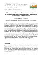
HYDROGEN BONDING

Hydrogen
atoms

104.5°

Figure 2-1
Hydrogen bonding between water
molecules.

The attractive interaction between a hydrogen atom of one
water molecule and the unshared electrons of the oxygen
atom in another water molecule is known as a hydrogen bond,
represented schematically on Fig. 2-1. Estimates of hydrogen
bond energy between molecules range from 10 to 40 kJ/mol,
which is approximately 1 to 4 percent of the covalent O–H
bond energy within a single molecule (McMurry and Fay,
2003). Hydrogen bonding causes stronger attractive forces
between water molecules than the molecules of most other
liquids and is responsible for many of the unique properties
of water.


2-1 Fundamental and Engineering Properties of Water

21

Compared to other species of similar molecular weight, water has higher
melting and boiling points, making it a liquid rather than a gas under
ambient conditions. Hydrogen bonding, as described above, can be used to
explain the unique properties of water including density, high heat capacity, heat of formation, heat of fusion, surface tension, and viscosity of water.
Examples of the unique properties of water include its capacity to dissolve a
variety of materials, its effectiveness as a heat exchange fluid, its high density
and pumping energy requirements, and its viscosity. In dissolving or suspending materials, water gains characteristics of biological, health-related,
and aesthetic importance. The type, magnitude, and interactions of these
materials affect the properties of water, such as its potability, corrosivity,
taste, and odor. As will be demonstrated in subsequent chapters, technology now exists to remove essentially all of the dissolved and suspended
components of water. The principal engineering properties encountered
in environmental engineering and used throughout this book are reported
in Table 2-1. The typical numerical values given in Table 2-1 are to provide
a frame of reference for the values that are reported in the literature.

Engineering
Properties
of Water

Table 2-1
Engineering properties of water
Valuea

Unit
Property

Symbol

SI
◦

C

U.S.
Customary
◦

SI

U.S.
Customary

F

100

212

Temperature at which vapor
pressure equals 1 atm; high value
for water keeps it in liquid state
at ambient temperature.
Pure water is not a good
conductor of electricity; dissolved
ions increase conductivity.

Definition/Notes

Boiling point

bp

Conductivity

κ

μS/m

μS/m

5.5

5.5

Density

ρ

kg/m3

slug/ft3

998.2

1.936

Dielectric
constant

εr

unitless

unitless

80.2

80.2

Measure of the ability of a solvent
to maintain a separation of
charges; high value for water
indicates it is a very good solvent.

Dipole moment

p

C •m

1.855

Measure of the separation of
charge within a molecule; high
value for water indicates it is very
polar.

D (debye) 6.186 × 10−30

(continues)

22

2 Physical and Chemical Quality of Water

Table 2-1 (Continued)
Valuea

Unit
SI

U.S.
Customary

SI

U.S.
Customary

Hf

kJ/mol

btu/lbm

−286.5

−6836

Energy associated with the
formation of a substance from
the elements.

Enthalpy
of fusionb

Hfus

kJ/mol

btu/lbm

6.017

143.6

Energy associated with the
conversion of a substance
between the solid and liquid
states (i.e., freezing or melting).

Enthalpy of
vaporizationc

Hv

kJ/mol

btu/lbm

40.66

970.3

Energy associated with the
conversion of a substance
between the liquid and gaseous
states (i.e., vaporizing or
condensing); high value for
water makes distillation very
energy intensive.

75.34

0.999

Energy associated with raising
the temperature of water by
one degree; high value for
water makes it impractical to
heat or cool water for municipal
treatment purposes.

Property
Enthalpy
of formation

Symbol

Heat capacityd

cp

Melting point

mp

J/mol • ◦ C btu/lbm • ◦ F

◦

◦

F

0

32

MW

g/mole

g/mole

18.016

18.016

Specific weight

γ

kN/m3

lbf /ft

9.789

62.37

Surface tension

σ

N/m

lbf /ft

0.0728

0.00499

2.339

0.34

Molecular
weight

C

3

2

Vapor pressure

pv

kN/m2

lbf /in

Viscosity,
dynamic

μ

N • s/m2

lbf • s/ft

Viscosity,
kinematic

ν

m2 /s

ft2 /s

2

Definition/Notes

Also known as molar mass.

1.002×10−3 2.089×10−5
1.004×10−6 1.081×105

values for pure water at 20◦ C (68◦ F) and 1 atm pressure unless noted otherwise.
the melting point (0◦ C).
c At the boiling point (100◦ C).
d Often called the molar heat capacity when expressed in units of J/mol • ◦ C and specific heat capacity or specific heat when
expressed in units of J/g • ◦ C.
e Molecular weight has units of Daltons (Da) or atomic mass units (AMU) when expressed for a single molecule (i.e., one mole
of carbon-12 atoms has a mass of 12 g and a single carbon-12 atom has a mass of 12 Da or 12 AMU).
a All
b At


2-2 Units of Expression for Chemical Concentrations

2-2 Units of Expression for Chemical Concentrations
Water quality characteristics are often classified as physical, chemical
(organic and inorganic), or biological and then further classified as health
related or aesthetic. To characterize water effectively, appropriate sampling
and analytical procedures must be established. The purpose of this section

is to review briefly the units used for expressing the physical and chemical
characteristics of water. The basic relationships presented in this section
will be illustrated and expanded upon in subsequent chapters. Additional
details on the subject of sampling, sample handling, and analyses may be
found in Standard Methods (2005).
Commonly used units for the amount or concentration of constituents
in water are as follows:
1. Mole:
6.02214 × 1023 elementary entities (molecules, atoms, etc.)
of a substance
1.0 mole of compound = molecular weight of compound, g (2-1)
2. Mole fraction: The ratio of the amount (in moles) of a given solute
to the total amount (in moles) of all components in solution is
expressed as
nB
xB =
(2-2)
nA + nB + nC + · · · + nN
where

xB
nA
nB
nC

= mole fraction of solute B
= moles of solute A
= moles of solute B
= moles of solute C
..

.

nN = moles of solute N

The application of Eq. 2-2 is illustrated in Example 2-1.
3. Molarity (M):
M , mol/L =

mass of solute, g
(molecular weight of solute, g/mol)(volume of solution, L)
(2-3)

4. Molality (m):
m, mol/kg =

mass of solute, g
(molecular weight of solute, g/mol)(mass of solution, kg)
(2-4)

23


24

2 Physical and Chemical Quality of Water

Example 2-1 Determination of molarity and mole fractions
Determine the molarity and the mole fraction of a 1-L solution containing
20 g sodium chloride (NaCl) at 20◦ C. From the periodic table and reference
books, it can be found that the molar mass of NaCl is 58.45 g/mol and the

density of a 20 g/L NaCl solution is 1.0125 kg/L.
Solution
1. The molarity of the NaCl solution is computed using Eq. 2-3
[NaCl] =

20 g
= 0.342 mol/L = 0.342 M
(58.45 g/mol)(1.0 L)

2. The mole fraction of the NaCl solution is computed using Eq. 2-2
a. The amount of NaCl (in moles) is
20 g
nNaCl =
= 0.342 mol
58.45 g/mol
b. From the given solution density, the total mass of the solution is
1012.5 g, so the mass of the water in the solution is 1012.5 g −
20 g = 992.5 g and the amount of water (in moles) is
nH 2 O =

992.5 g
= 55.08 mol
18.02 g/mol

c. The mole fraction of NaCl in the solution is
nNaCl
0.342 mol
xNaCl =
= 6.17 × 10−3
=

nNaCl + nH2 O
0.342 mol + 55.07 mol
Comment
The molar concentration of pure water is calculated by dividing the density
of water by the MW of water; i.e., 1000 g/L divided by 18 g/mol equals
55.56 mol/L. Because the amount of water is so much larger than the
combined values of the other constituents found in most waters, the mole
fraction of constituent A is often approximated as xA ≈ (nA /55.56). If this
approximation had been applied in this example, the mole fraction of NaCl
in the solution would have been computed as 6.16 × 10−3 .

5. Mass concentration:
Concentration, g/m3 =
Note that 1.0 g/m3 = 1.0 mg/L.

mass of solute, g
volume of solution, m3

(2-5)


2-3 Physical Aggregate Characteristics of Water

6. Normality (N):
N , eq/L =

mass of solute, g
(equivalent weight of solute, g/eq)(volume of solution, L)
(2-6)

where
molecular weight of solute, g/mol
Z , eq/mol
(2-7)
For most compounds, Z is equal to the number of replaceable hydrogen atoms or their equivalent; for oxidation–reduction reactions, Z is
equal to the change in valence. Also note that 1.0 eq/m3 = 1.0 meq/L.
7. Parts per million (ppm):
mass of solute, g
(2-8)
ppm = 6
10 g of solution
Also,
Equivalent weight of solute, g/eq =

ppm =

concentration of solute, g/m3
specific gravity of solution (density of solution divided by density of water)
(2-9)

8. Other units:
ppmm = parts per million by mass (for water ppmm = g/m3 = mg/L)
ppmv = parts per million by volume
ppb = parts per billion
ppt = parts per trillion
Also, 1 g (gram) = 1 × 103 mg (milligram) = 1 × 106 μg (microgram)
= 1 × 109 ng (nanogram) = 1 × 1012 pg (picogram).

2-3 Physical Aggregate Characteristics of Water
Most first impressions of water quality are based on physical rather than

chemical or biological characteristics. Water is expected to be clear, colorless, and odorless (Tchobanoglous and Schroeder, 1985). Most natural
waters will contain some material in suspension typically comprised of
inorganic soil components and a variety of organic materials derived from
nature. Natural waters are also colored by exposure to decaying organic
material. Water from slow-moving streams or eutrophic water bodies will
often contain colors and odors. These physical parameters are known as
aggregate characteristics because the measured value is caused by a number of individual constituents. Parameters commonly used to quantify the
aggregate physical characteristics include (1) absorption/transmittance,
(2) turbidity, (3) number and type of particles, (4) color, and (5)
temperature. Taste and odor, sometimes identified as physical characteristics, are considered in Sec. 2-6.

25


26

2 Physical and Chemical Quality of Water

Absorbance and
Transmittance

The absorbance of a solution is a measure of the amount of light that
is absorbed by the constituents in a solution at a specified wavelength.
According to the Beer–Lambert law, the amount of light absorbed by
water is proportional to the concentration of light-absorbing molecules
and the path length the light takes in passing through water, regardless
of the intensity of the incident light. Because even pure water will absorb
incident light, a sample blank (usually distilled water) is used as a reference.
Absorbance is given by the relationship
log

where

I
I0

= −ε(λ)Cx = −kA (λ)x = −A(λ)

(2-10)

I = intensity of light after passing through a solution
of known depth containing constituents of
interest at wavelength λ, mW/cm2
I 0 = intensity of incident light after passing through a
blank solution (i.e., distilled water) of known
depth (typically 1.0 cm) at wavelength λ, mW/cm2
λ = wavelength, nm
ε (λ) = molar absorptivity of light-absorbing solute at a
wavelength λ, L/mol · cm
C = concentration of light-absorbing solute, mol/L
x = length of light path, cm
kA (λ) = ε(λ)C = absorptivity at wavelength λ, cm−1
A(λ) = ε(λ)Cx = absorbance at wavelength λ, dimensionless

If the left-hand side of Eq. 2-10 is expressed as a natural logarithm, then
the right-hand side of the equation must be multiplied by 2.303 because
the absorbance coefficient (also known as the extinction coefficient) is
determined in base 10. Absorbance is measured using a spectrophotometer,
as illustrated on Fig. 2-2. Typically, a fixed sample path length of 1.0 cm
is used. The absorbance A(λ) is unitless but is often reported in units
of reciprocal centimeters, which corresponds to absorptivity kA (λ). If the

Photodetector at
90° for measuring
turbidity
Scattered light
Transmitted light

Aperture

Figure 2-2
Schematic of a spectrophotometer used
to measure absorbance and turbidity.

Light source

In-line photodetector
for measuring
absorbance and
transmittance

Lens

Incident light

Water sample in
glass cell


2-3 Physical Aggregate Characteristics of Water

length of the light path is 1 cm, absorptivity is equal to the absorbance. The

absorbance of water is typically measured at a wavelength of 254 nm. Typical
absorbance values for various waters at λ = 254 are given in Table 13-10.
The application of Eq. 2-10 is illustrated in the following example.

Example 2-2 Determine average UV intensity
If the intensity of the UV radiation measured at the water surface in a Petri
dish is 15 mW/cm2 , determine the average UV intensity to which a sample
will be exposed if the depth of water in the Petri dish is 12 mm (1.2 cm).
Assume the absorptivity kA (λ) = 0.1/cm.
Solution
1. Develop the equation to determine the average intensity.
a. The definition sketch for this problem is given below.
Intensity

Sample depth

0

I0

0

I = I0e−αx

dx

Iavg d
d
x

where

α = 2.303kA (λ)

b. Develop the required equation:

Iavg =

d
0

=−

Iavg =

I0 e

−αx

I
dx = − 0 e−αx
α

d

0

I0 αd I0
I
e + = 0 1 − e−αd

dα
α
α

I0
1 − e−αd
αd

27


28

2 Physical and Chemical Quality of Water

2. Compute the average intensity for a depth of 12 mm (1.2 cm):
a. Assume kA (λ) = 0.1/cm
b. α = 2.303 kA (λ) = 2.303 (0.1/cm) = 0.2303/cm
c. Solve for I avg

Iavg =

I0
15 mW/cm2
1 − e−(0.2303)(1.2)
1 − e−αd =
αd
(0.2303/cm)(1.2 cm)

= 13.1 mW/cm2

The transmittance of a solution is defined as
Transmittance, T , % =

I
I0

× 100

(2-11)

Thus, the transmittance at a given wavelength can also be derived from
absorbance measurements using the relationship
T = 10−A(λ)

(2-12)

The term percent transmittance, commonly used in the literature, is given as
T , % = 10−A(λ) × 100

(2-13)

The extreme values of A and T are as follows (Delahay, 1957):
For a perfectly transparent solution A(λ) = 0, T = 1.
For a perfectly opaque solution A(λ) → ∞, T = 0.
The principal water characteristics that affect the percent transmittance
include selected inorganic compounds (e.g., copper and iron), organic
compounds (e.g., organic dyes, humic substances, and aromatic compounds
such as benzene and toluene), and small colloidal particles (≤0.45 μm).
If samples contain particles larger that 0.45 μm, the sample should be

filtered before transmittance measurements are made. Of the inorganic
compounds that affect transmittance, iron is considered to be the most
important with respect to UV light absorbance because dissolved iron can
absorb UV light directly. Organic compounds containing double bonds and
aromatic functional groups can also absorb UV light. Absorbance values
for a variety of compounds are given in the on-line resources for this text
at the URL listed in App. E. The reduction in transmittance observed in
surface waters during storm events is often ascribed to the presence of
humic substances and particles from runoff, wave action, and stormwater
flows (Tchobanoglous et al., 2003).


2-3 Physical Aggregate Characteristics of Water

29

Turbidity in water is caused by the presence of suspended particles that
reduce the clarity of the water. Turbidity is defined as ‘‘an expression
of the optical property that causes light to be scattered and absorbed
rather than transmitted with no change in direction or flux level through
the sample’’ (Standard Methods, 2005). Turbidity measurements require a
light source (incandescent or light-emitting diode) and a sensor to measure
the scattered light. As shown on Fig. 2-2, the scattered light sensor is located
at 90◦ to the light source. The measured turbidity increases as the intensity
of the scattered light increases. Turbidity is expressed in nephelometric
turbidity units (NTU).
It is important to note that the scattering of light caused by suspended
particles will vary with the size, shape, refractive index, and composition
of the particles. Also, as the number of particles increases beyond a given
level, multiple scattering occurs, and the absorption of incident light is

increased, causing the measured turbidity to decrease (Hach, 2008). The
spatial distribution and intensity of the scattered light, as illustrated on
Fig. 2-3, will depend on the size of the particle relative to the wavelength of
the light source. For particles less than one-tenth of the wavelength of the
incident light, the scattering of light is fairly symmetrical. As the particle
size increases relative to the wavelength of the incident light, the light
reflected from different parts of the particle creates interference patterns
that are additive in the forward direction (Hach, 2008). Also, the intensity
of the scattered light will vary with the wavelength of the incident light.
For example, blue light will be scattered more than red light. Based on
these considerations, turbidity measurements tend to be more sensitive to

Turbidity

Suspended
particle
Incident light

(a)

Pattern of
light scatter

Incident light

(b)

Incident light

(c)

Figure 2-3
Light-scattering patterns for different particle sizes
that occur when measuring turbidity. (Adapted
from Hach, 2008.)


30

2 Physical and Chemical Quality of Water

particles in the size range of the incident-light wavelength (0.3 to 0.7 μm
for visible light). A further complication with turbidity measurements is
that some particles such as carbon black will essentially absorb most of the
light and only scatter a minimal amount of the incident light.
Depending on the water source, turbidity can be the most variable of the
water quality parameters of concern in drinking water supplies. Turbidity
measurements are useful for comparing different water sources or treatment facilities and are used for process control and regulatory compliance.
Increases in turbidity measurements are often used as an indicator for
increased concentrations of water constituents, such as bacteria, Giardia
cysts, and Cryptosporidium oocysts.
In lakes or reservoirs, turbidity is frequently stable over time and ranges
from about 1 to 20 NTU, excluding storm events. Turbidity in rivers is more
variable due to storm events, runoff, and changes in flow rate in the river.
Turbidity in rivers can range from under 10 to over 4000 NTU. Streams and
rivers where the turbidity can change by several hundred NTU in a matter
of hours (see Fig. 2-4) are often described as ‘‘flashing’’ because of the
rapid change in the turbidity. In such rivers, careful turbidity monitoring is
critical for successful process control. The regulatory standard for turbidity
in finished water is 0.3 NTU, and many water treatment facilities have a

treatment goal of <0.1 NTU, which is near the detection limit for turbidity
meters.
Particles

Particles are defined as finely divided solids larger than molecules but
generally not distinguishable individually by the unaided eye, although
300

Raw-water turbidity, NTU

250

200

1 : 1 blend of
river water and
reservoir water

150

100

Reservoir
source water

50

Figure 2-4
Observed variation in raw-water turbidity values.
(Adapted from James M. Montgomery, 1981.)

0

2 4 6 8 10 12 14 16 18 20 22 24 26 28 30
Time, d


2-3 Physical Aggregate Characteristics of Water

clumps of particles are often encountered. It should be noted that with
20–20 vision it is possible to resolve a particle size of about 37 μm at a
distance of 0.3 m. Particles in water are important for a variety of reasons,
including their impact on treatment processes and the potential health
impacts of pathogen-associated particles. Particles in water may be classified according to their source, size, chemical structure, electrical charge
characteristics, and water–solid interface characteristics. The source, size,
shape, number and distribution, and quantification of particles is considered in the following discussion. The electrical properties of particles and
particle interactions are considered in Chap. 9. The impact of particles in
water on key water treatment processes, that is, coagulation, sedimentation,
granular filtration, membrane filtration, and disinfection, is considered in
Chaps. 9, 10, 11, 12, and 13, respectively.
SOURCE OF PARTICLES IN WATER

The sources of particles in water are summarized in Table 2-2, along with
the sources of chemical constituents and gases. As reported in Table 2-2, the
principal natural sources of particles in water are soil-weathering processes
and biological activity. Clays and silts are produced by weathering. Algae,
bacteria, and other higher microorganisms are the predominant types
of particles produced biologically. Some particles have both natural and
anthropogenic sources, a notable example being asbestos fibers. Industrial
and agricultural activities tend to augment these natural sources by increasing areas of runoff through cultural eutrophication, the increase in the rate

of natural eutrophication as a result of human activity, or direct pollution
with industrial residues. Particles may be transported into water through
direct erosion from terrestrial environments, be suspended due to turbulence and mixing in water, or form in the water column during biological
activity or chemical precipitation or through atmospheric deposition.
SIZE CLASSIFICATION OF PARTICLES

The size of particles in water considered in this text is typically in the
range of 0.001 to 100 μm. Suspended particles are generally larger than
1.0 μm. The size of colloidal particles will vary from about 0.001 to
1 μm depending on the method of quantification. It should be noted that
some researchers have classified the size range for colloidal particles as
varying from 0.0001 or less to 1 μm. In practice, the distinction between
colloidal and suspended particles is blurred because the suspended particles
that can be removed by gravity settling will depend on the design of the
sedimentation facilities. Some standard analytical procedures operationally
define dissolved material as that which will pass through a 0.45 μm filter.
In practice, however, colloids as small as 0.001 μm can behave as particles
and affect water quality and treatment processes as particles rather than
dissolved substances. A suspension comprised of particles of one size is

31


32

Decompostion
of organic matter
in environment

Rain in contact

with atmosphere

Contact of water
with minerals,
rocks, and soil
(e.g., weathering)

Source

Various organic polymers

Cell fragments

Clay, silt, sand,
Clay
and other
Silica (SiO2 )
inorganic soils
Ferric oxide (Fe2 O3 )
Aluminum oxide (Al2 O3 )
Magnesium dioxide (MnO2 )

Particulate constituents
Colloidal
Suspended

Bicarbonate (HCO− )
Chloride (Cl− )
2−
Sulfate (SO4 )

Bicarbonate (HCO− )
Chloride (Cl− )
Hydroxide (OH− )
−
Nitrate (NO3 )
−
Nitrite (NO2 )
Sulfide (HS− )
2−
Sulfate (SO4 )

Ammonium (NH4+ )
Hydrogen (H+ )
Sodium (Na+ )

Phosphate (PO4 )
2−
Sulfate (SO4 )

3−

Carbonate (CO3 )
Chloride (Cl− )
Fluoride (F− )
Hydroxide (OH− )
−
Nitrate (NO3 )

2−

Bicarbonate (HCO− )
−
Borate (H2 BO3 )

Hydrogen (H+ )

Calcium (Ca2+ )
Iron (Fe2+ )
Magnesium (Mg2+ )
Manganese (Mn2+ )
Potassium (K+ )
Sodium (Na+ )
Zinc (Zn2+ )

Ionic and Dissolved Constituents
Positive ions
Negative ions

Ammonia (NH3 )
Carbon dioxide (CO2 )
Hydrogen sulfide (H2 S)
Hydrogen (H2 )
Methane (CH4 )
Nitrogen (N2 )
Oxygen (O2 )
Silicate (H4 SiO4 )

Carbon dioxide (CO2 )
Nitrogen (N2 )
Oxygen (O2 )

Sulfur dioxide (SO2 )

Carbon dioxide (CO2 )
Silicate (H4 SiO4 )

Gases and Neutral
Species

Table 2-2
Summary of important particulate, chemical, and biological constituents found in water according to their source


33

Inorganic and organic
solids, constituents
causing color, chlorinated
organic compounds,
bacteria, worms, viruses,
etc.

Municipal,
industrial,
and agricultural
sources and other
human activity
Clay, silt, grit, and
other inorganic
solids; organic
compounds; oil;

corrosion
products; etc.

Algae, diatoms,
minute animals,
fish, etc.

Source: Adapted, in part, from Tchobanoglous and Schroeder (1985).

Bacteria, algae, viruses,
etc.

Living organisms

Inorganic ions,
including a variety
of anthropogenic
compounds and
heavy metals

—

Ammonia (NH3 )
Carbon dioxide (CO2 )
Hydrogen sulfide (H2 S)
Hydrogen (H2 )
Methane (CH4 )
Nitrogen (N2 )
Oxygen (O2 )

Inorganic ions,
Chlorine (Cl2 )
Sulfur dioxide (SO2 )
including a variety
of anthropogenic
compounds, organic
molecules, color, etc.

—


34

2 Physical and Chemical Quality of Water

called monodispersed and a suspension with a variety of particle sizes is
called heterodispersed (typical of natural waters).
Many water treatment processes are designed to remove particles based
on sedimentation and size exclusion. The type and size of various waterborne particles and processes used for measurement and removal are
presented on Fig. 2-5. As shown on Fig. 2-5, conventional treatment processes such as sedimentation and depth filtration alone are not sufficient
for the removal of all water constituents; however, with the addition of coagulation and flocculation, the effective range of these treatment processes is
greatly extended.
PARTICLE SHAPE

Particle shapes found in water can be described as spherical, semispherical,
ellipsoids of various shapes (e.g., prolate and oblate), rods of various length
and diameter, disk and disklike, strings of various lengths, and random coils.
Inorganic particles are typically defined by the dimensions of their long,
intermediate, and short axes and the ratio of the intermediate-to-long and
the short-to-intermediate diameters. Because of the many different particle

shapes, the nominal or equivalent particle diameter is used (Dallavalle,
1948). Large organic molecules are often found in the form of coils that
may be compressed, uncoiled, or almost linear. The shape of some larger
particles is often described as fractal. The particle shape will vary depending
on the characteristics of the source water.
PARTICLE QUANTIFICATION

Methods used for the quantification and analysis of particulate material include gravimetric techniques, electronic particle size counting, and
microscopic observation. Although regulations concerning particle concentrations are typically based on turbidity measurements, monitoring particle
counts throughout a treatment process can aid in understanding and controlling the process. Also, as noted above, turbidity measurements cannot
be correlated to any quantifiable particle characteristics. While particle
quantification may be useful for evaluating a treatment process, except
for microscopic observation, these methods cannot be used reliably for
determining the source or type of particle (e.g., distinguish between a
viable cyst and a colloid). In addition, due to the limitations of particle
analysis methods, the use of more than one method is recommended when
assessing water quality data.
Gravimetric techniques
The total mass of particles may be estimated by filtering a volume of water
through a membrane of known weight and pore size. Filtration of the same
water sample through a series of membranes with incrementally decreasing
pore sizes is known as serial filtration. Serial filtration may be used to
determine an approximate particle size distribution (Levine et al., 1985).


2-3 Physical Aggregate Characteristics of Water

35

Approximate molecular mass, amua

101

102

103

104

105

106

107

Synthetic organic compounds

Water
constituents

Nutrients

Fulvic acids

Amino acids

Fatty acids

Algae

Polysaccharides

Bacteria

Cell fragments

RNA

Carbohydrates

109

Viruses

Humic acids

Chlorophyll

108

Organic debris and bacterial flocs

DNA

Proteins

Cryptosporidium oocysts
Clay particles

Exocellular enzymes

Vitamins

Giardia lamblia cysts

Colloidal material

Silt particles
Depth filtration

Treatment
processes

Activated carbon pores

Microfiltration
Ultrafiltration

Nanofiltration

Sedimentation

Reverse osmosis

Analytical
separation

Gel filtration chromatography

Sedimentation
Centrifugation

High-pressure liquid chromatography

Sieves
Membrane filter technique

Ultrafiltration molecular sieves

Suspended solids test
Coulter counter

Measurement
and visulaization

HiAC particle counter
Laser light scattering
Light microscopy
Electron microscopy
Human vision

Scanning tunneling microscopy

0.0001

0.001

0.01

0.1

1

10

100

Particle size, μm
aAn amu is an atomic mass unit (also known as a dalton, Da) and is equal to 1.66054 × 10−24 g.
Figure 2-5
Characterization of particulate matter in natural water by type and size, appropriate treatment methods, analytical separation
methods, and measurement techniques. (Adapted from Tchobanoglous et al., 2003.)


36

2 Physical and Chemical Quality of Water

Particle size distribution may also be measured using electronic particlecounting devices, as discussed below.
Electronic particle size counting
Particle concentration measurements provide more specific information
about the size and number of particles in a water sample. Electronic
particle size counters estimate the particle size concentration by either (1)
passing a water sample through a calibrated orifice and measuring the
change in conductivity (see Fig. 2-6) or (2) passing the sample through a
laser beam and measuring the change in intensity due to light scattering.
The change in conductivity or light intensity is correlated to the diameter of
an equivalent sphere. Particle counters have sensors available in different
size ranges, such as 1.0 to 60 μm or 2.5 to 150 μm, depending on the
manufacturer and application. Particle counts are typically measured and
recorded in about 10 to 20 subranges of the sensor range. Typical particle

size counters are shown on Fig. 2-7. A comparison of analytical techniques
used for particle size analysis is presented in Table 2-3. Particle counts may
also be used as an indicator of Giardia and Cryptosporidium cysts from water
(LeChevallier and Norton, 1992, 1995).
Microscopic observation
The use of microscopic observation allows for the determination of particle
size counts and, in some cases, for more rigorous identification of a particle’s

Particles

Ruby orifice
embedded in glass

Electrodes used to
measure voltage
differences as particles
pass through orifice

Figure 2-6
Typical particle-counting chamber
used to enumerate particles in water
using voltage difference to
determine the size of an equivalent
spherical particle. (Adapted from
Tchobanoglous et al., 2003.)

Fluid containing
particles to be
counted flows
through orifice

Voltage difference
and thickness of orifice
used to determine
equivalent spherical
diameter of particle


2-3 Physical Aggregate Characteristics of Water

(a)

(b)

Table 2-3
Analytical techniques used for analysis of particles in water
Technique
Microscopy
Light
Transmission electron
Scanning electron
Image analysis
Particle counting
Conductivity difference
Dynamic light scattering
Equivalent light scattering
Light obstruction (blockage)
Light diffraction
Separation
Centrifugation

Field flow fractionation
Gel filtration chromatography
Gravitation photosedimentation
Sedimentation
Membrane filtration

Typical Size Range, μm
0.2–>100
0.0002–>0.1
0.002–50
0.2–>100
0.2–>100
0.0003–5
0.005–>100
0.2–>100
0.3–>100
0.08–>100
0.09–>100
<0.0001–>100
0.1–>100
0.05–>100
0.0001–1

Source: Adapted from Levine et al. (1985).

origin than is possible with other analysis techniques. A measured volume
of sample is placed in a particle-counting cell and the individual particles
may be counted, often with the use of a stain to enhance the particle
contrast. Optical imaging software may also be used to obtain a more
quantitative assessment of particle characteristics. Images of water particles

are obtained with a digital camera attached to a microscope and sent to
a computer for imaging analysis. The imaging software typically allows for

37
Figure 2-7
Typical examples of
particle size counters are
(a) laboratory type
connected to a computer
(the sample to be
analyzed is being
withdrawn from the
graduated cylinder) and
(b) field type used to
monitor the particle size
distribution from a
microfiltration plant.


38

2 Physical and Chemical Quality of Water

the determination of minimum, mean, and maximum size, shape, surface
area, aspect ratio, circumference, and centroid location.
PARTICLE NUMBER AND DISTRIBUTION

The number of particles in raw surface water can vary from 100 to over
10,000/mL depending on the time of year and location where the sample
is taken (e.g., a river or storage reservoir). The number of particles, as will

be discussed later, is of importance with respect to the method to be used
for their removal. The size distribution of particles in natural waters may be
defined on the basis of particle number, particle mass, particle diameter,
particle surface area, or particle volume. In water treatment design and
operation, particle size distributions are most often determined using a
particle size counter, as discussed above. In most particle size counters,
the detected particles of a given size are counted and grouped with other
particles within specified size ranges (e.g., 1 to 2 μm, 5 to 10 μm). When
the counting is completed, the number of particles in each bin is totaled.
The particle number frequency distribution F (d) can be expressed as
the number concentration of particles, dN , with respect to the incremental
change in particle size, d(dp ), represented by the bin size:
F (dp ) =

dN
d(dp )

(2-14)

where F (dp ) = function defining frequency distribution of particles d1 ,
d2 , d3
dN = particle number concentration with respect to
incremental change in particle diameter d(dp )
d(dp ) = incremental change in particle diameter (bin size)
Because of the wide particle size ranges encountered in natural waters,
it is common practice to plot the frequency function dF(d) against the
logarithm of size, log dp :
2.303(dp )F (d) =

dN

d(log dp )

(2-15)

Similar relationships can be derived based on particle surface area and
volume (Dallavalle, 1948; O’Melia, 1978).
It has also been observed that in natural waters the number of particles increases with decreasing particle diameter and that the frequency
distribution typically follows a power law distribution of the form
dN
= A dp
d(dp )

−β

N
(dp )

(2-16)


2-3 Physical Aggregate Characteristics of Water

where

39

A = power law density coefficient
dp = particle diameter, μm
β = power law slope coefficient

Taking the log of both sides of Eq. 2-16 results in the following expression,
which can be plotted to determine the unknown coefficients A and β:
log

N / (dp ) = log A − β log(dp )

(2-17)

The value of A is determined when dp = 1 μm. As the value of A increases,
the total number of particles in each size range increases. The slope β is
a measure of the relative number of particles in each size range. Thus,
if β < 1, the particle size distribution is dominated by large particles; if
β = 1, all particle sizes are represented equally; and if β > 1, the particle
size distribution is dominated by small particles (Trussell and Tate, 1979).
The value of the coefficient for most natural waters varies between 2 and
5 (O’Melia, 1978; Trussell and Tate, 1979). Typical plots of particle size
data determined using a particle size counter for various waters are given
on Fig. 2-8. On Fig. 2-8a, the effect of flocculation in producing large
particles is evident by comparing the β values for the unflocculated versus
the flocculated influent (4.1 versus 2.1). As shown on Fig. 2-8b, the removal
of all particle sizes by filtration is very similar, because the slopes of the two
plots are nearly identical. The analysis of data obtained from a particle size
counter is shown in Example 2-3.

4

5

3
log[ΔN/Δ(dp)]

log[ΔN/Δ(dp)]

2
1
0
−1

Unflocculated
water, β = 4.1

−2
1

10
100
Particle size dp, μm
(a)

Filter
influent,
β = 4.1

4

Flocculated
water, β = 2.1

3
2

1
0
−1

Filter
effluent,
β = 4.1

1

2 10 20
50
Particle size dp, μm
(b)

150

Figure 2-8
Typical examples of
particle size distributions:
(a) unflocculated and
flocculated and (b) filter
influent and effluent.
(Adapted from Trussell
and Tate, 1979.)


40

2 Physical and Chemical Quality of Water

Example 2-3 Analysis of particle size information
Determine the slope and density coefficients A and β in Eq. 2-17 for the
following particle size data obtained from settled water during a pilot study.
Channel (Bin)

Particle size range, μm

Number of Particles, #/mL

1
2
3
4
5
6

1–3
3–5
5–7
7–12
12–32
32–120
Total

1785
243
145
186
132

2.9
2493.9

Solution
1. Calculate the necessary values for the first data channel.
a. Mean particle diameter:
dp =

1
2

1 μm + 3 μm = 2 μm

b. Log of the mean particle diameter:
log dp = log 2 μm = 0.301
c. Particle diameter range:
dp = 3 μm − 1 μm = 2 μm
d. Number of particles:
N = 1785/mL
e. Log of the particle size distribution function:
log

N
dp

= log

1785/mL
2 μm

= 2.95

2. Calculate the necessary values for the remaining data channels. The
results are tabulated below.
Channel

(A)
dp

(B)
log (dp )

(C)
Δ(dp )

(D)
ΔN

1
2
3
4
5
6

2
4
6
9
22

76

0.301
0.602
0.778
0.978
1.342
1.881

2
2
2
5
20
88

1785
243
145
186
132
2.9

(E)
log [ΔN/Δ(dp )]
2.95
2.08
1.86
1.57
0.82

−1.48


2-3 Physical Aggregate Characteristics of Water

41

3. Prepare a plot of log[ N / (dp )] versus log(dp ) draw a linear trendline
and display the treadline equation and r2 value on the chart. The
resulting chart is shown below.
4
y = −2.65x + 3.90
r 2 = 0.96

log [ΔN/Δ(dp)]

3
2
1
0
−1
−2

0

0.5

1
log (dp)

1.5

2

4. Determine A and β in Eq. 2-17 from the line of best fit in the above
plot.
a. When log(dp ) = 0, the intercept value is equal to log(A). Thus,
A = 7,940.
b. The slope of the line of best fit is equal to −β. Thus, β = 2.65.

The color of a water is an indication of the organic content, including
humic and fulvic acids, the presence of natural metallic ions such as iron
and manganese, and turbidity. Apparent color is measured on unfiltered
samples and true color is measured in filtered samples (0.45-μm filter).
Turbidity increases the apparent color of water, while the true color is
caused by dissolved species and is used to define the aesthetic quality of
water. The color of potable waters is typically assessed by visually comparing
a water sample to known color solutions made from serial dilutions or concentrations of a standard platinum–cobalt solution. The platinum–cobalt
standard is related to the color-producing substance in the water only
by hue.
The presence of color is reported in color units (c.u.) at the pH of the
solution. In water treatment, one of the difficulties with the comparison
method is that at low levels of color it is difficult to differentiate between
low values (e.g., 2 versus 5 c.u.). If the water sample contains constituents
(e.g., industrial wastes) that produce unusual colors or hues that do not
match the platinum–cobalt standards, then instrumental methods must be

Color