Lighting information
Bạn đang xem bản rút gọn của tài liệu. Xem và tải ngay bản đầy đủ của tài liệu tại đây (147.95 KB, 16 trang )
CSC418 / CSCD18 / CSC2504
12
Radiometry and Reflection
Radiometry and Reflection
Until now, we have considered highly simplified models and algorithms for computing lighting and
reflection. These algorithms are easy to understand and can be implemented very efficiently; however, they also lack realism and cannot achieve many important visual effects. In this chapter, we
introduce the fundamentals of radiometry and surface reflectance that underly more sophisticated
models. In the following chapter, we will describe more advanced ray tracing algorithms that take
advantage of these models to produce very realistic and simulate many real-world phenomena.
12.1 Geometry of lighting
In our discussion of lighting and reflectance we will make several simplifying assumptions. First,
we will ignore time delays in light propagation from one place to another. Second, we will assume
that light is not scattered nor absorbed by the median through which it travels, e.g., we will ignore
light scattering due to fog and other atmospheric effects. These assumptions allow us to focus on
the geometry of lighting; i.e., we can assume that light travels along straight lines, and is conserved
as it travels (e.g., see Fig. 1).
Light Tube
B
A
Figure 1: Given a set of rays within a tube, passing through A and B but not the sides of the tube,
the flux (radiant power) at A along these rays is equal to that at B along the same set of rays.
Before getting into the details of lighting, it will be useful to introduce three key geometric concepts, namely, differential areas, solid angle and foreshortening. Each of these geometric concepts
is related to the dependence of light on the distance and orientation between surfaces in a scene
that receive or emit light.
Area differentials: We will need to be able describe the amount of lighting hitting an area on a
surface or passing through a region of space. Integrating functions over a surface requires that we
introduce an area differential over the surface, denoted dA. Just as a 1D differential (dx) represents
an infinitesimal region of the real line, an area differential represents an infinitesimal region on a
2D surface.
Example:
Consider a rectangular patch S in the x − y plane. We can specify points in the patch
in terms of an x coordinate and a y coordinate, with x ∈ [x0 , x1 ], y ∈ [y0 , y1 ]. We can
Copyright c 2005 David Fleet and Aaron Hertzmann
76
CSC418 / CSCD18 / CSC2504
Radiometry and Reflection
divide the plane into N M rectangular subpatches, the ij-th subpatch bounded by
xi ≤ x ≤ xi + ∆x
yj ≤ y ≤ yj + ∆y
(1)
(2)
where i ∈ [0...N − 1], j ∈ [0...M − 1], ∆x = (x1 − x0 )/N and ∆y = (y1 − y0 )/M .
The area of each subpatch is Ai,j = ∆x∆y. In the limit as N → ∞ and M → ∞,
dA = dxdy
(3)
To compute the area of a smooth surface S, we can break the surface into many tiny
patches (i, j), each with area Ai,j , and add up these individual areas:
Area(S) =
Ai,j
(4)
i,j
In the planar patch above, the area of the patch is:
Area(S) =
Ai,j = N M ∆x∆y = (x1 − x0 )(y1 − y0 )
(5)
i,j
Computing these individual patch areas for other surfaces is difficult. However, taking the infinite limit as the area of the patches decreases, we get the general formula:
Area(S) =
dA
(6)
S
For the planar patch, this becomes:
y1
x1
dA =
S
dxdy = (x1 − x0 )(y1 − y0 )
y0
(7)
x0
We can create area differentials for any smooth surface. Fortunately, in most radiometry applications, we do not actually need to be able to do so for anything other than a plane. We will use area
differentials when we integrate light on the image sensor, which, happily, is planar. However, area
differentials are essential to many key definitions and concepts in radiometry.
Solid angle: We need to have a measure of angular extent in 3D. For example, we need to be
able to talk about what we mean by the field of view of a camera, and we need a way to quantitfy
the width of a directional light (e.g., a spot light).
Copyright c 2005 David Fleet and Aaron Hertzmann
77
CSC418 / CSCD18 / CSC2504
Radiometry and Reflection
Let’s consider the situation in 2D first. In 2D, angular extent is just the angle between two directions, and we normally specify angular extent in radians. The angular extent between two rays
emanating from a point q¯ can be measured using a circle centered at q¯; that is, the angular extent
(in radians) is just the circular arc length l of the circle between the two directions, divided by
radius r of the circle, l/r (see Fig. 2). For example, the angular extent of an entire circle having
circumference 2πr is just 2π radians. A half-circle has arclength πr and spans π radians.
l
r
q
Figure 2: Angular extent in 2D is given by l/r (radians).
In 3D, the quantity corresponding to 2D angular extent is called solid angle. Analogous to the 2D
case, solid angle is measured as the area a of a patch on a sphere, divided by the squared radius of
the sphere (Figure 3); i.e.,
a
(8)
ω = 2
r
The unit of measure for solid angle is the steradian (sr). A solid angle of 2π steradians corresponds
to a hemisphere of directions. The entire sphere has a solid angle of 4π sr. As depicted in Figure
3, to find the solid angle of a surface S with respect to a point q¯, one projects S onto a sphere of
radius r, centered at q¯, along lines through q¯. This gives us a, so we then divide by r2 to find the
solid angle subtended by the surface. Note that the solid angle of a patch does not depend on the
radius r, since the projected area a is proportional to r2 .
a
q
S
r
Figure 3: The solid angle of a patch S is given by the area a of its projection onto a sphere of radius
r, divided by the squared radius, r2 .
Note:
At a surface point with normal n, we express the hemisphere of incident and emittant
directions in spherical coordinates. That is, directions in the hemisphere d are
d = (sin θ cos φ, sin θ sin φ, cos θ)T
Copyright c 2005 David Fleet and Aaron Hertzmann
(9)
78
CSC418 / CSCD18 / CSC2504
Radiometry and Reflection
where θ ∈ [0, π/2] denotes the angle between d and the surface normal, and φ ∈
[−π, π) specifies the direction projected onto the surface.
With direction expressed in this way one can write the infinitesimal solid angle as
dω = sin θ dθ dφ
(10)
The infinitesimal solid angle is an area differential for the unit sphere.
To see this, note that for θ held fixed, if we vary φ we trace out a circle of radius sin θ
that is perpendicular to n. For a small change dφ, the circular arc has length sin θ dφ,
and therefore the area of a small ribbon of angular width dθ is just sin θ dθ dφ.
dq
sinq
sin q dj
q
1
dj
With differential solid angle we can now compute the finite solid angle for a a range
of visual direction, such as θ0 ≤ θ ≤ θ1 and φ0 ≤ φ ≤ φ1 . That is, to compute
the solid angle we just integrate the differential solid angle over this region on a unit
sphere (r = 1):
φ1
θ1
ω =
sin θ dθ dφ
φ0
φ1
=
φ0
(11)
θ0
− cos θ|θθ10 dφ
= (φ1 − φ0 )(cos θ0 − cos θ1 )
(12)
(13)
(Assuming we are in the quadrant where this quantity is positive)
Foreshortening: Another important geometric property is foreshortening, the reduction in the
(projected) area of a surface patch as seen from a particular point or viewer. When the surface
normal points directly at the viewer its effective size (solid angle) is maximal. As the surface
normal rotates away from the viewer it appears smaller (Figure 4). Eventually when the normal
is pointing perpendicular to the viewing direction you see the patch “edge on”; so its projection is
just a line (with zero area).
Putting it all together: Not surprisingly, the solid angle of a small surface patch, with respect to
a specific viewing location, depends both on the distance from the viewing location to the patch,
Copyright c 2005 David Fleet and Aaron Hertzmann
79
CSC418 / CSCD18 / CSC2504
A θ
Radiometry and Reflection
q
~ A cos θ
dA θ
r
q
dA cosθ
Figure 4: Foreshortening in 2D. Left: For a patch with area A, seen from a point q¯, the patch’s
foreshortened area is approximately A cos θ. This is an approximation, since the distance r varies
over the patch. The angle θ is the angle between the patch normal and the direction to q¯. Right:
For an infinitesimal patch with area dA, the foreshortened area is exactly dA cos θ.
and on the orientation of the patch with respect to the viewing direction.
Let q¯ be the point (such as a light source or a viewer) about which we want to compute solid angle.
Let p¯ be the location of a small planar surface patch S with area A at distance r = ||¯
q − p¯|| from
q¯. Additionally, suppose the surface normal points directly at q¯ (Figure 5). In this case, we can
imagine drawing a hemisphere about q¯ with radius r, and the projected area a of this patch will be
approximately A. Hence, the solid angle ω ≈ A/r2 . In other words, the solid angle is inversely
proportional to distance squared; a more distant object obscures less of q¯’s “field of view.” This is
an approximation, however, since the distance r varies over the patch. Nevertheless, if we consider
the limit of an infinitesimal patch with area dA, then the solid angle is exactly dω = dA/r2 .
When the surface normal does not point directly at q¯, foreshortening plays a significant role. As
the surface normal rotates away from the direction of q¯ − p¯, the surface, as viewed from point q¯,
becomes smaller; it projects onto a smaller area on a sphere centered at q¯. sphere. So, we say that
the area of the patch, as seen from q¯, is foreshortened. More formally, let θ be the angle between
the normal n and direction, q¯ − p¯. Then, for our infinitesimal surface with area dA, the solid angle
subtended by the tilted patch is
dA cos θ
dω =
,
(14)
r2
The cosine term should look familiar; this is the same cosine term used in Lambertian shading
within the Phong model.
12.2 Elements of Radiometry
The field of radiometry concerns the measurement of light (electromagnetic radiation), usually
restricted to the visible wavelengths, in the range 400-700 nm. Light is often measured in discrete
units called photons. It is difficult to talk about the number of photons that illuminate a point
on a surface at a particular time (as it is almost always zero). Instead, we talk about the average
number of photons in small (infinitesimal) intervals of space or time, that is, we talk about photon
density, and thereby treat light as a continuous quantity rather than a photon count. In effect, we
are assuming that there is enough light in the scene so that we can treat light as a continuous
function of space-time. For example, we will talk about the light hitting a specific surface patch as
a continuous function over the patch, rather than discuss the discrete photons of light.
Copyright c 2005 David Fleet and Aaron Hertzmann
80
CSC418 / CSCD18 / CSC2504
Radiometry and Reflection
q
q
Figure 5: Solid angle of a patch. Left: A patch with normal pointing at ¯l. Right: A patch with
arbitrary orientation.
12.2.1
Basic Radiometric Quantities
Formally, we describe light in terms of radiant energy. You can think of radiant energy as the
totality of the photons emitted from a body over its entire surface and over the entire period of
time it emits light. Radiant energy is denoted by Q(t) and measured in Joules (J). You can think of
radiant energy as describing how much light has been emitted from (or received by) a surface up
to a time t, starting from some initial time 0. 1
The main quantity of interest in radiometry is power, that is, the rate at which light energy is
emitted or absorbed by an object. This time-varying quantity, usually called flux, is measured in
Joules per second (J · s−1 ). Here we denote flux by Φ(t):
Φ(t) =
dQ(t)
dt
(15)
We can compute the total light that hits a surface up to time t as:
t
Φ(τ ) dτ
Q(t) =
(16)
0
Flux is sufficiently important that we define a special unit of measure for it, namely, watts (W).
One watt is one Joule per second; so a 50 watt light bulb draws 50J of energy per second. Most
of this radiant energy is emitted as visible light. The rest is converted to thermal energy (heat).
Higher wattage means a brighter light bulb.
Not surprisingly, the light received or emitted by an object varies over the surface of the object.
This is important since the appearance of an object is often based on how the light reflected from
1
Of course, radiant energy depends on wavelength λ, so it is common to express energy as a function of wavelength;
the resulting density function, Q(λ), is called spectral energy. This is important since different wavelengths are seen
as different colours. Nevertheless, our next major simplification will be to ignore the dependence of radiant energy on
wavelength. In computer graphics, colours are controlled by the relative amounts of power in three separate spectral
bands, namely, Red, Green, and Blue. What we describe in this chapter can be applied to each colour channel.
Copyright c 2005 David Fleet and Aaron Hertzmann
81
CSC418 / CSCD18 / CSC2504
Radiometry and Reflection
its surface depends on surface position. Formally, light received at the surface of an object, as a
function of image position is called irradiance. The light emitted from a surface, as a function of
surface position, is often called radiant exitance (or radiosity).
Irradiance, the incident flux, as a function of surface position p¯, is denoted by H(¯
p). Remember,
we cannot talk about the amount of light received at a single point on a surface because the number
of photons received at a single point is generally zero. Instead, irradiance is the spatial density of
flux, i.e., the amount of light per unit surface area. The integral of irradiance over the surface of an
object gives us the total incident flux (i.e., received by) the object. Accordingly, irradiance is the
spatial derivative of flux. For smooth surfaces we write
H(¯
p) =
dΦ
dA
(17)
where dA refers to differential surface area. Irradiance is just power per unit surface area (W·m−2 ).
Example:
For a planar patch in the x − y plane, we can write irradiance as a function of (x, y)
position on the patch. Also, we have dA = dxdy. In this case:
H(x, y) =
d2 Φ
dxdy
(18)
These terms are all functions of time t, since lighting Φ may change over time t. However, we will
leave the dependence on time t implicit in the equations that follow for notational simplicity.
Example:
What is the irradiance, owing to a point light source, on an infinitesimal patch
S with area dA? Let’s say we have a point light source at ¯l emitting I watts per
steradian into all directions:
dΦ = Idω
(19)
In other words, the amount of light from this source is proportional to solid angle,
and independent of direction. Our goal is to compute the irradiance H on the patch,
which can be done by subtitution of formulas from this chapter:
H =
dΦ
Idω
IdA cos θ
I cos θ
=
=
=
2
dA
dA
dAr
r2
(20)
where p¯ is the position of S, r = ||¯l − p¯||, and θ is the angle between the surface
normal and the vector ¯l − p¯. This formula illustrates the importance of solid angle:
the amount of light hitting a surface is proportional to its solid angle with respect to
Copyright c 2005 David Fleet and Aaron Hertzmann
82
CSC418 / CSCD18 / CSC2504
Radiometry and Reflection
the light source. A distant patch (with large r) receives less light than a nearby patch,
and a foreshortened patch receives less light than a frontal patch. Furthermore, the
amount of light hitting the patch is proportional to the intensity I of the light source.
12.2.2
Radiance
Of course the light emitted or received by an object depends on visual direction as well as surface
position. For example, objects are often illuminated more from above (the sky) than below (the
ground). As a consequence, when the direction of light propagation is important, we will express
flux as a function of visual direction. This leads to the central quantity in radiometry, namely,
radiance. Radiance is a measure of the rate at which light energy is emitted from a surface in
a particular direction. It is a function of position and direction, and it is often denoted by L (or
L(¯
p, d)). Formally, it is defined as power per steradian per surface area (W · sr−1 · m−2 ), where the
surface area is defined with respect to a surface patch at p¯ that is perpendicular to the direction d.
Normally, one might think of radiance as a measure of the light emitted from a particular surface
location into a particular direction. The definition above is more general however. It allows us to
talk about the light travelling in a particular direction through an arbitrary point in space. In this
case we are measuring surface area with respect to a virtual surface, but we can talk about surface
area nonetheless.
When we talk about the light (radiance) emitted from a particular surface into a particular emittant
direction de we have to be a little more careful because radiance is defined with respect to a surface
perpendicular to the emittant direction, which is usually not the same orientation as the actual real
surface in question. Accordingly, often radiance is defined as power per unit foreshortened surface
area per solid angle to make explicit the fact that we are using a virtual surface and not the real
surface to measure area. That is, we are measuring surface area as seen by someone looking at the
surface from somewhere along a ray in the emittant direction.
de
dA = cos θ dAs
n
de
dω
θ
dAs
dAs
Note:
Computing radiant exitance (radiosity): As mentioned above, radiant exitance is
the total amount of flux leaving a surface into the entire hemisphere of emittant diCopyright c 2005 David Fleet and Aaron Hertzmann
83
CSC418 / CSCD18 / CSC2504
Radiometry and Reflection
rections, as a function of surface position. Intuitively, it is the integral of surface
radiance, but we have to be careful; radiance is defined with respect to unit area on
a surface perpendicular to the emittant direction rather than unit area on the real surface of interest. Before we can integrate radiance we need to specify all radiance
quantities in terms of unit surface area on the real surface. To do this one needs to
multiply radiance for emittant direction de by the ratio of the surface area normal
to de (i.e., dA), to the real surface area, denoted dAs . As discussed above, for an
infinitesimal patch the ratio of these areas is just the foreshortening factor, i.e.,
dA = cos θ dAs = n · de dAs ,
(21)
where θ is the angle between the unit vectors n and de .
Taking this foreshortening factor into account, the relation between radiant exitance
E(¯
p) and radiance L(¯
p, d) is given by
L(¯
p, d) n · d dω
E(¯
p) =
(22)
d∈Ωe
The domain of integration, Ωe , is the hemisphere of possible emittant directions.
Note:
Computing Irradiance: Above we showed that the irradiance on an infinitesimal
surface patch S at point p¯ owing to a point light source at q¯ with radiant intensity I
is given by
H =
I cos θ
r2
(23)
where r = ||¯
q − p¯|| is the distance between the light source and the surface patch,
and θ is the angle between the surface normal and the direction of the light source
from the surface patch, q¯ − p¯.
In this case, the radiance at p¯ from the point light source direction d = p¯ − q¯/r, i.e.,
L(¯
p, d), is simply I/r2 . The factor cos θ is the foreshortening factor to convert from
area perpendicular to the direction d to area on the surface S.
Accordingly, if we consider radiance at p¯ from the entire hemisphere of possible
incident directions, then the total irradiance at p¯ is given by
L(¯
p, −d) n · d dω
H(¯
p) =
(24)
d∈Ωi
(Note that incident directions here are outward facing from p¯.)
Copyright c 2005 David Fleet and Aaron Hertzmann
84
CSC418 / CSCD18 / CSC2504
Radiometry and Reflection
Note:
Radiance vs. Irradiance. Radiance and irradiance are very similar concepts — both
describe an amount of light transmitted in space — but it is important to recognize the
distinctions between them. There are several ways of thinking about the difference:
• Radiance is a function of direction; it is power per foreshortened surface area
per steradian in a specific direction. Irradiance is incident power per surface
area (not foreshortened); it is not a directional quantity.
• Radiance (W · sr−1 · m−2 ) and irradiance (W · m−2 ) have different units.
• Radiance describes light emitted from a surface. Irradiance describes light incident on a surface. Indeed, from the radiance emitted from one surface we can
compute the incident irradiance at a nearby surface.
12.3 Bidirectional Reflectance Distribution Function
We are now ready to explore how to model the reflectance properties of different materials. Different objects will interact with light in different ways. Some surfaces are mirror-like, while others
scatter light in a wide variety of directions. Surfaces that scatter light often look matte, and appear
similar from different viewing directions. Some objects absorb a significant amount of light; the
colour of an object is largely a result of which wavelengths it absorbs and which wavelengths it
reflects.
One simple model of surface reflectance is refered to as the bidirectional reflectance distribution
function (BRDF). The BRDF describes how light interacts with a surface for a relatively wide
range of common materials. In intuitive terms, it specifies what fraction of the incoming light from
a given incident direction will be reflected toward a given emittant direction. When multiplied by
the incident power (i.e., the irradiance), one obtains the desired emittant (i.e., reflected) power.
More precisely, the BRDF is a function of emittant and incident directions de and di . It is defined
to be the ratio of radiance to irradiance:
ρ(de , di ) =
L
H
(25)
For most common materials the only way to determine the BRDF is with measurements. That is,
for a wide range of incident and emittant directions, a material is illuminated from one direction
while the reflected light is measured from another direction. This is often a tedious procedure.
In computer graphics it is more common to design (i.e., make up) parametric BRDF formulae,
and then vary the parameters of such models to achieve the desired appearance. Most parametric
models are based on analytic models of certain idealized materials, as discussed below.
Copyright c 2005 David Fleet and Aaron Hertzmann
85
CSC418 / CSCD18 / CSC2504
Radiometry and Reflection
12.4 Computing Surface Radiance
When rendering an image of an object or scene, one wants to know how much light is incident at
each pixel of the image plane. (In effect, one wants to compute the image irradiance.) Fortunately
it can be shown that this quantity is linearly related to the scene radiance. In particular, for a point
on an opaque object in a given visual direction, one simply needs to compute the radiance from
that point on the surface in the direction of the camera. Based on the BRDF model of reflectance,
the surface radiance depends on the incident illumination (irradiance) at the surface, and the BRDF
of course.
Point Light Sources
For example, consider a single point source with radiant intensity I. To compute the irradiance
at a small surface patch we can compute the total flux arriving at the surface, and then divide by
the area of the surface to find flux per unit area. More precisely, radiant intensity for the source is
given by I = dΦ/dω. We multiply by the solid angle subtended by the patch dω to obtain the flux
on the surface dΦ, and then we divide by the surface area dA to obtain dΦ/dA, that is, irradiance
as in Eqn (17). For a point light source this was shown above (see Eqn. (20)) to be given by
H = I
n · di
r2
(26)
where n is the unit surface normal, di is the unit vector in the direction of hte light source from the
surface patch, and r is the distance from the patch to the light source.
We now want to compute the radiance from the surface (e.g., toward the camera). Toward this end,
we multiply the irradiance H by the BRDF, ρ(de , di ), in order to find radiance as a function of the
emittant direction:
n · di
(27)
L(¯
p, de ) = ρ(de , di ) I 2
r
This perspective generalizes naturally to multiple light sources. That is, the radiance from a point
p on a surface in the direction of the camera is the sum of radiances due to individual light sources.
For J point light sources, at locations lj , with intensities Ij , the radiance is given by
J
L(¯
p, de ) =
ρ(de , dj ) Ij
j=1
n · dj
rj2
(28)
where rj = ||¯lj − p¯|| is the distance to the j th source, and dj = (¯lj − p¯)/rj is the incident direction
of the j th source.
Copyright c 2005 David Fleet and Aaron Hertzmann
86
CSC418 / CSCD18 / CSC2504
Radiometry and Reflection
Extended Light Sources
Many light sources are not infinitesimal point sources. Rather, in the general case we need to be
able to work with extended light sources for which the incident light is a continuous function of
incident direction. One way to think of this is to let the number of discrete light sources go to
infinity so that the sum in Eqn (28) becomes an integral.
Here we take a slightly different, but equivalent approach. As discussed above, radiance can be
used to express the light energy transport through any point in space, in any direction of interest.
Thus, given a point p¯ on a surface with unit normal n, we can express the radiance through p¯ along
the hemisphere of possible incident directions as L(¯
p, di ) for di ∈ Ωi where Ωi denotes the domain
of plausible incident directions at p¯.
Note:
As above, we can erect a spherical coordinate system at p¯. Toward this end, let θi
denote an angle measured from the surface normal, and let φi be an angle in the
surface tangent plane about the normal relative to some Cartesian x − y coordinate
system in the plane. Then all directions
di ≡ (sin θi cos φi , sin θi sin φi , cos θi )T
(29)
contained in Ωi satisfy θi ∈ [0, π/2] and φi ∈ [−π, π).
One problem with radiance is the fact that it expresses the light flux in terms of power per unit
area on a surface perpendicular to the direction of interest. Thus, for each incident direction we are
using a different plane orientation. In our case we want to express the power per unit area on our
surface S, and therefore we need to rescale the radiance in direction di by the ratio of foreshortened
surface area to surface area. One can show that this is accomplished by multiplying L(¯
p, di ) by
cos θi = di · n, for normal n. The result is now the incident power per unit surface area (not
foreshortened) per solid angle. We multiply this by solid angle dω to obtain irradiance:
H = L(¯
p, −di ) cos θi dωi
(30)
Therefore, the resulting surface radiance in the direction of the camera due to this irradiance is just
ρ(de , di ) L(¯
p, −di ) cos θi dωi
If we then accumulate the total radiance from the incident illumination over the entire hemisphere
of possible incident directions we obtain
ρ(de , di ) L(¯
p, −di ) cos θi dωi
L(de ) =
(31)
di ∈Ωi
Copyright c 2005 David Fleet and Aaron Hertzmann
87
CSC418 / CSCD18 / CSC2504
Radiometry and Reflection
where, as above, the infinitesimal solid angle is dωi = sin θi dθi dφi .
Light sources vary greatly from scene to scene. In effect, when you take a photograph you are
measuring irradiance at the image plane of the camera for a limited field of view (angular extent).
This shows how complex illumination sources can be.
Note:
The ideal point light source can also be cast in the framework of a continuous, extended source. To do this we assume that the distribution of incident light can be
modeled by a scaled Dirac delta function. A Dirac delta function δ(x) is defined by:
δ(x) = 0 for x = 0 , and
δ(x) f (x) dx = f (0)
(32)
x
With the light source defined as a delta function, Eqn (31) reduces to Eqn (27).
12.5 Idealized Lighting and Reflectance Models
We now consider several important special instances of BRDF models. In particular, we are interested in combinations of lighting and BRDF models that facilitate efficient shading algorithms.
We discuss how diffuse and specular surfaces can be represented as BRDFs.
12.5.1
Diffuse Reflection
A diffuse (or matte) surface is one for which the pattern of shading over the surface appears the
same from different viewpoints. The ideal diffusely reflecting surface is known as a perfect Lambertian surface. Its radiance is independent of the emittant direction, its BRDF is a constant, and
it reflects all of the incident light (i.e., it absorbs zero power). The only factor that determines the
appearance (radiance) of a Lambertian surface is therefore the irradiance (the incident light). In
this case, with the BRDF constant, ρ(de , di ) = ρ0 , the (constant) radiance Le has the form:
L(¯
p, −di ) cos θi dωi
Ld (¯
p, de ) = ρ0
(33)
di ∈Ωi
Note:
A perfect Lambertian surface reflects all incident light, absorbing none. Therefore,
the total irradiance over the hemisphere of incident directions must equal the radiant
exitance. Setting these quantities to be equal, one can show that ρ0 = 1/π. The
BRDF for any diffuse surface must therefore have a value between 0 and 1/π.
Despite the simplicity of the BRDF, it is not that simple to compute the radiance because we still
have an integral over the hemisphere of incident directions. So let’s simplify the model further.
Copyright c 2005 David Fleet and Aaron Hertzmann
88
CSC418 / CSCD18 / CSC2504
Radiometry and Reflection
Let’s assume a single point light source with intensity I at location ¯l. This gives us
Ld (¯
p, de ) = ρ0 I
n · di
r2
(34)
where r = ||¯l − p¯|| is the distance to the light source from p¯, and di = (¯l − p¯)/r is the direction of
the source from p¯. Of course, the surface normal n also changes with p¯.
Eqn (34) is much easier to compute, but we can actually make the computation even easier. Let’s
assume that the point source is sufficiently far away that r and di do not change much with points
p¯ on the object surface. That is, let’s treat them as constant. Then we can simplify Eqn (34) to
Ld (¯
p) = rd I s · n
(35)
where rd is often called the diffuse reflection coefficient, and s is the direction of the source. Then
the only quantity that depends on surface position p¯ is the surface normal n.
Note:
The value s · n should actually be max(0, s · n). Why? Consider the relationship of
the light source and surface when this dot product is negative.
12.5.2
Ambient Illumination
The diffuse shading model in Eqn (34) is easy to compute, but often appears artificial. The biggest
issue is the point light source assumption, the most obvious consequence of which is that any
surface normal pointing away from the light source (i.e., for which s · n < 0) will have a radiance
of zero. A better approximation to the light source is a uniform ambient term plus a point light
source. This is a still a remarkably crude model, but it’s much better than the point source by itself.
With a uniform illuminant and a constant BRDF, it is easy to see that the integral in Eqn (33)
becomes a constant. That is, the radiance does not depend on the orientation of the surface because
the illumination is invariant to surface orientation. As a result we can write the radiance under a
uniform illuminant as
La (¯
p ) = r a Ia
(36)
where ra is often called the ambient reflection coefficient, and Ia denotes the integral of the uniform
illuminant.
Note:
If the illuminant is the sum of a point source and a uniform source, then the resulting
radiance is the sum of the radiances to the individual sources, that is, the sum of Eqns
(36) and (35).
Copyright c 2005 David Fleet and Aaron Hertzmann
89
CSC418 / CSCD18 / CSC2504
12.5.3
Radiometry and Reflection
Specular Reflection
For specular (mirror) surfaces, the incident light from each incident direction di is reflected toward
a unique emittant direction de . The emittant direction lies in the same plane as the incident direction
di and the surface normal n, and the angle between n and de is equal to that between n and di . One
n
de
di
can show that the emittant direction is given by de = 2(n · di )n − di . For all power from di be
reflected into a single emittant direction the BRDF for a perfect mirror must be proportional to a
delta function, ρ(de , di ) ∝ δ(di − (2(n · de )n − de )).
In particular, if we choose the constant of proportionality so that the radiant emittance is equal to
the total incident power, then the BRDF becomes:
ρ(de , di ) =
1
n · di
δ(di − (2(n · de )n − de ))
(37)
In this case, Eqn (31) reduces to
Ls (¯
p, de ) = L(¯
p, −(2(n · de )n − de ))
(38)
This equation plays a major role in ray tracing.
Off-Axis Specularity: Many materials exhibit a significant specular component in their reflectance. But few are perfect mirrors. First, most specular surfaces do not reflect all light, and
that is easily handled by introducing a scalar constant in Eqn (38) to attenuate surface radiance Ls .
Second, most specular surfaces exhibit some form of off-axis specular reflection. That is, many
polished and shiny surfaces (like plastics and metals) emit light in the perfect mirror direction and
in some nearby directions as well. These off-axis specularities look a little blurred. Good examples
are highlights on plastics and metals.
The problem with off-axis specularities is that the BRDF is no longer a simple delta function. The
radiance into a particular emittant direction will now be affected from the incident power over a
range of incident directions about the perfect specular direction. This means that, unlike the simple
radiance function in Eqn (38) for perfect measures, we need to return to the integral in Eqn (31).
Therefore it is not easy to compute radiance in this case.
Like the diffuse case above, one way to simplify the model with off-axis specularities is to assume
a point light source. With a point light source we can do away with the integral. In that case the
Copyright c 2005 David Fleet and Aaron Hertzmann
90
CSC418 / CSCD18 / CSC2504
Radiometry and Reflection
light from a distant point source in the direction of s is reflected into a range of directions about
the perfect mirror directions m = 2(n · s)n − s. One common model for this is the following:
Ls (de ) = rs I max(0, m · de )α ,
(39)
where rs is called the specular reflection coefficient (often equal to 1 − rd ), I is the incident power
from the point source, and α ≥ 0 is a constant that determines the width of the specular highlights.
As α increases, the effective width of the specular reflection decreases. In the limit as α increases,
this becomes a mirror.
12.5.4
Phong Reflectance Model
The above components, taken together, give us the well-known Phong reflectance model that was
introduced earlier:
L(¯
p, de ) = rd Id max(0, s · n) + ra Ia + rs Is max(0, m · de )α ,
(40)
where
• Ia , Id , and Ir are parameters that correspond to the power of the light sources for the ambient,
diffuse, and specular terms;
• ra , rd and rs are scalar constants, called reflection coefficients, that determine the relative
magnitudes of the three reflection terms;
• α determines the spread of the specurlar highlights;
• n is the surface normal at p¯;
• s is the direction of the distant point source;
• m is the perfect mirror direction, given n and s ; and
• and de is the emittant direction of interest (usually the direction of the camera).
Copyright c 2005 David Fleet and Aaron Hertzmann
91